Heuristic methods, for global optimization, have been receiving much interest in the last years, among which Particle Swarm Optimization (PSO) algorithm can be highlighted. However, the application of heuristic methods can lead to premature convergence. In this work, the addition of a step on the PSO algorithm is proposed. This new step, based in Nelder–Mead simplex search method (NM), consists of repositioning the current particle with global best solution, not for a better position, but away from the current nearest local optimum, to avoid getting stuck on this local optimum. There are other PSO-NM algorithms, but the one we are proposing, has a different strategy. The proposed algorithm was also tested with the repositioning strategy in other particles beyond the current global best particle, depending on the repositioning probability. To evaluate the effectiveness of the proposed methods, and study its better parameters, were used various test functions, and for each test function, various number of particles were used in combination with various probabilities of particles repositioning. A thousand runs were performed for each case, resulting in more than two millions runs. The computational studies showed that the repositioning of of global best particle increases the percentage of success on reaching the global best solution, but better results can be obtained applying the repositioning strategy to other particles with repositioning probabilities between 1–5%.
Keywords
particle swarm optimization
Nelder–Mead simplex search
unconstrained optimization
hybrid optimization method
global optimum
Author information
Introduction
Function minimization (or maximization) is extensively employed in various science fields. It refers to determination of the decision variables of a function, so that the function would be at its minimum (or maximum) value. A majority of problems, especially engineering ones, are optimization problems (function minimization or maximization) in which the decision variables should be determined in a way, that the systems will operate at their best operation points in relation to a specific objective [1]. Since most engineering and other science fields problems are non-linear, complicated and with various local optima, it is necessary to use methods with good ability of finding global optima. No method guarantees convergence to the global optimum, but recently a lot of heuristic methods have been proposed, and this class of methods present great potential in obtaining the global optimum.
The heuristic optimization methods are mostly inspired by nature as evolutionary, physical based, or based on animals or human behavior. The common characteristic among these models is that a global search is executed using movements of the search points, which is driven by a vector quantity given by its dynamic system, such as the distance to the best position already reached by all points [2]. The various methods include Simulated Annealing [3], Differential Evolution [4], Artificial Chemical Reaction Optimization Algorithm [5], Water Evaporation Optimization Algorithm [6], Lightning Search Algorithm [7], Lightning Attachment Procedure Optimization [1], Gravitational Search Algorithm [8], Black Hole Algorithm [9], Particle Swarm Optimization [10], Multi-Particle Collision Algorithm [11], Firefly Algorithm [12], Crow search algorithm [13], Whale Optimization Algorithm [14], Monkey Search Algorithm [15], Bat-inspired Algorithm [16], Artificial Bee Colony algorithm [17], Grey Wolf Optimization algorithm [18], Fruit Fly algorithm [19], Dragonfly algorithm [20], Social Spider Optimization [21], Cuckoo Optimization Algorithm [22], Lion Optimization Algorithm [23], Tabu Search [24, 25], League Championship Algorithm [26], Soccer League Competition Algorithm [27], Fireworks Algorithm [28], Colliding Bodies Optimization [29], Tug of War Optimization [30], Thermal Exchange Optimization [31], Ions Motion Algorithm [32], Pathfinder Algorithm [33], Black Widow Optimization Algorithm [34], Turbulent Flow of Water-based Optimization [35], and many others.
Immature convergence and stagnation at local minimum are some common deficiencies in the majority of heuristic optimization methods. Hence, researchers are often concerned to improve them through modifying previous optimizers, for example, modification on: Grey Wolf Optimization algorithm [36], Bat Algorithm [37], Particle Swarm Optimization [38–43], Firefly Algorithm [44], Fruit Fly Algorithm [45], Ant Colony Algorithm [46], Artificial Bee Colony [47–49], and so on.
It is difficult to predict the best algorithm for every optimization problem. However, a hybrid method of different optimization algorithms could be a potential solution and more efficient than using one single algorithm for solving complex problems [50]. Hybridization of heuristic algorithms with other heuristic or deterministic algorithms has been an active research area in recent years. For example, Particle Swarm Optimization and Simulated Annealing [51], Particle Swarm Optimization and Genetic Algorithm [52, 53], Particle Swarm Optimization and Support Vector Machines [54], Particle Swarm Optimization, Ant Colony Optimization and 3-Opt algorithms [55], Artificial Bee Colony Algorithm and Differential Evolution [56], Gravitational Search Algorithm and Genetic Algorithm [57], Extended Random Search and Conjugate Gradient Method [58], Scatter Search and Nelder–Mead [59], Genetic Algorithm and Newton Method [60], Simulated Annealing and Genetic Algorithm [61], Simulated Annealing and Tabu Search Algorithm [62], Particle Swarm Optimization, Spider Monkey Optimization and Ageist Spider Monkey Optimization algorithms [63], Whale Optimization Algorithm, Lévy Flight and Differential Evolution [64], Particle Swarm Optimization and Gravitational Search Algorithm [65], etc. Other hybrid methods are obtained by combining, in many ways, the Nelder–Mead simplex search (NM) and Particle Swarm Optimization (PSO), proposed respectively by Nelder and Mead [66] and Kennedy and Eberhart [10]. These methods are commonly called PSO-NM [67–72].
The focus in this work is to use a hybrid PSO-NM method for solving unconstrained optimization problems. The idea is to add a step in PSO algorithm where the particle with current global best value is repositioned, by a simplex methodology (the simplex is formed by the current global best and other particles) taking it away from the current nearest local minimum. This aims to avoid the global best particle from getting stuck in a local minimum, resulting in a premature convergence. This repositioning strategy is applied to another particles beyond the global best. The effectiveness of the proposed method is evaluated by computational studies comparing the rate of successful on reaching the global minimum for many test functions.
Literature review
Over the past few decades, heuristic algorithms have been increasingly popular in dealing with challenging optimization problems in all kinds of engineering fields. This is because such techniques are more inexpensive and efficient than conventional numerical approaches. The merits of heuristics lie in many aspects. The first is their randomness, which can ensure success in avoiding local extrema and exploring the search space. The second is the black box concept, in which the input and output of considered problems are used without the need of gradient information. In addition, heuristic algorithms are easy to implement and their mathematical models are simple [73].
Heuristic methods have gained popularity. They are approximate non-deterministic optimization techniques that draw on specialized knowledge to address a particular issue. Then, from heuristics, meta-heuristic algorithms emerged. They trended and appeared as an attempt to acquire strategies for problem-independent decision making. Meta-heuristic algorithms are created to address a variety of optimization problems by directing the search process and trying to explore the search area fully. They have a greater level of abstraction than heuristics, allowing for the incorporation and management of many heuristics as well as the integration of methods for escaping from local optima to reach the global optimum [74]. The advantages and disadvantages of various meta-heuristic algorithms are mentioned in brief.
Evolutionary Programming (EP) is simple to implement and suitable for many problems, but there is an uncertainty on determining the best resolution. Differential Evolution (DE) does not become stuck in a local minimum but the tuning parameters need improvement. Genetic Algorithm (GA) has good coverage of initial solutions in the search space, but the convergence is slow [74]. Another advantage of GA over traditional optimization is its treatment of more practical, dynamic, and highly nonlinear problems.
Bio-inspired optimization (BIO) easily copes with failure and consequently, real-world engineering challenges. The BIO system always finds the best solution. However, broadening the range and development of bioinspired methods for analysing new areas of application is necessary to overcome one of its drawbacks, which is the lack of balance amongst its elements [74–76].
Jaya Algorithm is a human-based and can be used to solve numerous optimization challenges. However, Jaya algorithm might be stuck in local optima when trying to address complex optimization issues because of minimal population information in its only learning strategy [77].
Teaching learning-based optimization (TLBO) has the capacity to balances global search capability with convergence rate and the ability for local and global search, but the exploration process needs to be improved. Social evolution and learning optimization (SELO) is effective in finding global optimum solutions for unconstrained problems, however has a relatively slow convergence speed. Gravitational search algorithm (GSA) can explore the local solution and is simple to implement, nonetheless, has a poor convergence rate and high computational time [74]. Although GSA surpasses traditional PSO and GA approaches in many issues, there are still some shortcomings such as exploration–exploitation discrepancy and local convergence [78].
Water Cycle Algorithm (WCA) is an effective population based optimization algorithm, but the algorithm still resorts to premature convergence or gets stuck in local optima in attempting to solve problems and requires a substantial calculation time [78, 79]. An evaluation of several tests provides varying levels of complexity that confirm the effectiveness of the electromagnetism optimization (EMO) technique regarding accuracy, speed and consistency [21, 74]. Multiverse Optimizer Algorithm (MVO) requires less effort in computation, however the algorithm gets stuck in the local optimal solution [74]. Sine Cosine Algorithm (SCA) solves a large variety of optimization challenges, has the ability to look into diverse areas of a search space, avoiding local optima, converging towards global optimization and searching for promising regions on the search space [74, 80].
By combining the two phases (fusion and fission), Nuclear Reaction Optimization (NRO) maintains a balance between its exploration and exploitation abilities. The tests indicated that this optimization method is a potentially powerful and an efficient global optimization algorithm [74].
Among heuristic intelligent optimization algorithms, swarm heuristic intelligence optimization algorithms have been widely used to solve global optimization problems due to simplicity, flexibility, and high efficiency. By introducing randomness in the optimization process, swarm intelligence optimization algorithms can determine the global optimal solution accurately and reasonably, which makes the solution of swarm intelligence optimization algorithm have practical significance [81]. Among heuristic intelligence optimization, Particle Swarm Optimization (PSO) is one of the most widely used; it is a simple, easy to implement, effective but can get stuck on local minimum and is unsatisfactory in solving multi-objective optimization problems [74].
Although several novel metaheuristics and solvers have been published and made available, the need to develop robust and intelligent systems is the need of the hour. This can be achieved by combining the known advantages of conventional methods with novel strategies or designing hybrid algorithms [82].
PSO-NM hybrid methods
The PSO-NM method proposed by Liu and Yang [70] uses the NM search method to improve the efficiency of PSO by increasing the convergence rate. This method, in each iteration, applies NM search method with a simplex composed by each particle and other n particles with best fitness value. Following this, all particles will be closer to the nearest local optimum. To justify the methodology proposed, the authors says that PSO method resists easily falling into local optimum, what is not entirely true, as will became clear later in this work. The method proposed by Liu and Yang [70] is a modification of the method proposed by Zahara and Hu [69], in which the NM method is applied in just one simplex, for each iteration, composed by n + 1 particles with best fitness value to improve the position of (n + 1)th particle, and other particles position are adjusted by PSO by taking in account the position of all particles used in the NM method.
Fan et al. [67] proposed a hybridization strategy of combining NM and PSO methods in a way to accelerate convergence. For an n dimensional problem, the procedure proposed by the authors uses 3 n + 1 particles, the particles are sorted by fitness, and the best n particles are saved for subsequent use. The top n + 1 particles are fed into the modified simplex search method to improve the (n + 1)th particle. Joined by the n best particles and the (n + 1)th particle, the last 2 n particles are adjusted by the modified PSO method.
The PSO-NM hybrid approach proposed by Hsu and Gao [68] aims to improve both convergence rate and accuracy of the proposed optimization algorithm, using an enhanced NM method to improve Gbest position and the help of a center particle, because the center particle is generally closer to the optimum than Gbest during the search. Due to frequent appearance as the best particle of swarm, it often attracts other particles and guides the search direction of the whole swarm, improving the convergence rate.
A PSO-NM method for crack detection in cantilever beams was proposed by Vakil Baghmisheh et al. [71], and used by Mesbahi et al. [72] in order to obtain the optimal parameters for Li-ion batteries model for vehicles. The hybrid PSO-NM is made-up of a modified particle swarm optimization algorithm (PSO), aimed at identifying the most promising areas, and a NM simplex algorithm for performing local search within these areas. For the modification of PSO method, a mutation operator is incorporated, in each iteration two randomly selected particles are deleted and two new particles are introduced and positioned randomly in the search space. In addition, to increase the precision of the answer the authors added the NM local search algorithm after the PSO.
Proposed new algorithm
The optimization techniques can be classified into two categories: deterministic (e.g., NM simplex search method, Steepest descent, Powell’s conjugate direction method, Rosenbrock method, etc.) and heuristic (e.g., PSO, simulated annealing algorithm, genetic algorithm, firefly algorithm, etc.). The advantage of deterministic methods is the lower computational time required, but for heuristic methods the probability of reaching the global minimum is greater. So the idea of this work is to propose an improvement of PSO method by using a repositioning methodology, of some particles, using the simplex approach proposed by Nelder and Mead [66], to avoid premature convergence provoked by the particles stuck in a local minimum, i. e., an hybridization strategy, to further increase the probability of global optimization success. The NM, PSO and PSO-NM (that we propose) methods are presented below.
Particle swarm optimization (PSO)
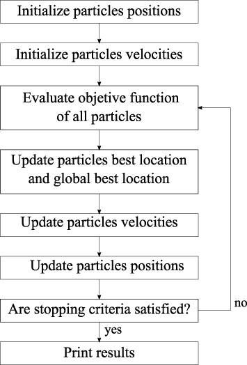
The Particle Swarm Optimization algorithm is based on the movement of organisms in a bird flock or fish school motivated by social exchange of information. Birds and fish adjust their physical moment to avoid predator, seek food, mate, optimize environmental parameters as temperature, etc. Humans adjust not only physical movement but cognitive or experiential variable as well [10]. So, the idea of this method is to randomly generate a swarm of m points (called “particles”), in the search region of dimension n, with initial random velocities. The function value of each particle are evaluated at each iteration. These function values are used to update particles velocities. It can be used to solve unconstrained as well as constrained optimization problems [83].
Figure 1.
PSO algorithm.
The procedure of PSO algorithm, illustrated by the figure 1, is composed of the following steps:
Positions initialization: randomly generate the initial positions (Xi) of m particles, within the limits of the n-dimensional search region. Considering that the search region has an upper bound, Xupper, and a lower bound, Xlower, a possible way to initialize the position is:
where rand() is a n-dimensional vector of random numbers between 0 and 1.
Velocities initialization: randomly generate the initial velocities (Vi) of m particles. It is not recommended that initial velocities have large values, so a possible way is to initialize as zero for all particles, another way is using the equation (2);
Evaluate objective function: for each current particle position, it is also called fitness (objective function value, Fobj);
Identify the best locations: for each particle, compare current objective function value with its best value reached ever, so, if current value is better than previous one, attribute particles best location (Pbest) is equal to current value. Identify the best value of objective function obtained with the current particles position, and compare it with previous global best location (Gbest), if the current value is better, update it;
Update particles velocities: the particles velocities are updated by equation (3);
where, w is the inertia weight, C1 is the cognitive parameter and C2 is the social parameter. Generally C1 = C2 = 2 and the inertia weight can be calculated by many equations, among which, the one commonly used is represented by equation (4) [84];
Update particles positions: the particles positions are updated by applying equation (5);
Stop condition: if stopping criteria was reached, go to step (8), otherwise return to step (3); In this work we used two stopping criteria, the iterative process is interrupted when one of then is satisfied. The stopping criteria are:
A large number of consecutive iterations (5000) with no changes larger than 1 × 10⁻⁷ in the value of objective function evaluated for Gbest;
All particles are very close to the Gbest:
Print results: print the position of global best location and its fitness as the minimum reached.
Nelder–Mead simplex search method (NM)
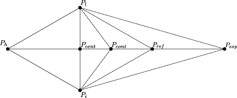
The idea of simplex method for function minimization of n variables without constraints, proposed by Nelder and Mead [66] based on an ingenious idea introduced by Spendley et al. [85], by comparing the function values at n + 1 vertices of a general simplex, followed by the replacement of the vertex with the highest objective function value by another point. This replacement is made until finding an approximation of local minimum.
In this method, initially, n + 1 points, i.e., P0, P1, P2, … , Pn are considered with function values, y0, y1, y2, … , yn respectively. So, the point with highest function value is defined as yh = max(yi) at Ph, the point with lowest function value as yl = min(yi) at Pl and the centroid, Pcent, of all points with i ≠ h. At each iteration a new simplex is formed by substituting Ph by reflection, contraction or expansion (these are illustrated in figure 2). The first operation consists in choosing a point, with lower function value than yh, away from Ph through Pcent by applying reflection equation (6)
where the reflection coefficient, 𝛼, is a positive constant (usually 𝛼 = 1).
Figure 2.
Nelder–Mead simplex substitution of Ph.
If the function value of Pref is lower than yl, i.e., the reflection resulted in a new minimum, so it is possible to obtain a function value even lower by applying expansion equation (7).
where the expansion coefficient, 𝛾, is a positive coefficient greater than unity (usually 𝛾 = 2).
If the function value at Pexp is lower than the function value at Pl, the new simplex is formed by replacing Ph by Pexp, otherwise Ph is replaced by Pref.
If a point, obtained on reflection operation, with a function value of Pref lower than yh and at least another one yi, Ph is replaced by Pref, otherwise if the fitness of Pref is higher than yi for all i ≠ h, it has obtained a new maximum. In this case, it is necessary to try taking a better new point by contraction, what is done by applying equation (8).
where the contraction coefficient, 𝛽, lies between 0 and 1 (usually 𝛽 = 1∕2). The value of Pcont is accepted unless the function value at this point remains higher than the values at Ph. In case the contraction fails, the simplex vertices are substituted applying equation (9).
PSO method with particle repositioning based on NM simplex (PSO-NM)
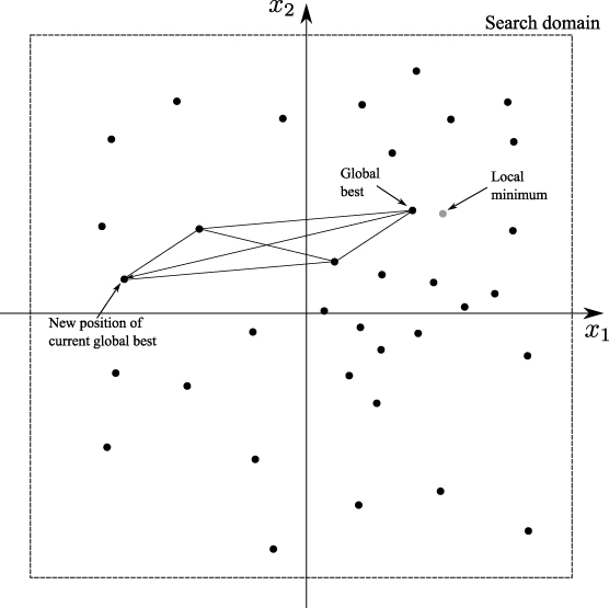
The PSO method we propose has a different purpose from all PSO-NM methods presented before. Starting from the possibility of one particle, at the beginning of optimization process, gets closer to a local minimum, this can attract other particles to this local minimum, and lead the algorithm to converge to this value, in other words, a premature convergence. An attempt to avoid getting stuck in a local minimum, we propose in this work, is using the reflection of NM simplex search method for the particle with global best fitness ever reached. As illustrated in figure 3, this reflection, of current global best particle, is done through a center obtained by n particles after (randomly chosen). This reflection operation takes the particle to a position away from current nearest local minimum, aiming to avoid getting stuck on local optimum.
Figure 3.
Repositioning of particle with current global best location.
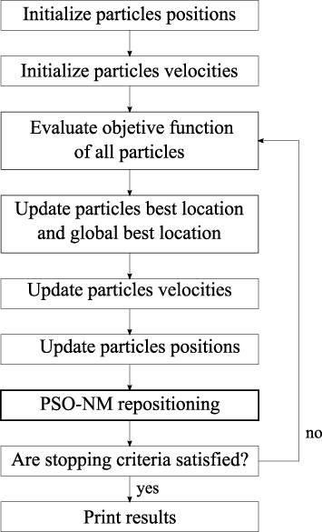
But the repositioning of just one particle cannot be satisfactory, aiming to fix this, we propose that this repositioning operation by NM reflection can occur, depending on a probability of particles repositioning, in other particles beyond that with global best fitness. This additional of repositioning, can improve the ability of avoiding premature convergence, besides that can aid better exploration of the search domain. This procedures are done after the update of positions (step 6) of PSO algorithm, as shown in figure 4.
Figure 4.
Proposed PSO-NM algorithm.
Numerical simulations methodology
The numerical simulations were implemented through two codes in ForTran. In the first code the PSO method was implemented, as presented in subsection 3.1, to obtain the minimal function value, and the possibility to use any number of particles. The proposed PSO-NM heuristic optimization method was implemented, as presented in subsection 3.3, in a way that the user can choose the number of particles and the probability of particles repositioning.
For both methods, we used simultaneously two stopping criteria, the first one verifies if, for too many iterations (5000), the value change in the global best fitness is less than the tolerance (tol = 1 × 10⁻⁷), and the last one verifies if all particles are so close to current global best (a distance less than the tolerance, tol = 1 × 10⁻⁷). If at least one of these stopping criteria is reached, the optimization method terminated successfully.
To make the comparison of effectiveness between PSO and the proposed PSO-NM method, we used various test functions (presented in Appendix A, where most of them have various local minima), where for each test function, were used various numbers of particles (5, 7, 10, 15, 20, 30, 40, 50, 100, 200, 300 and 500) and, for the PSO-NM method, were applied various probabilities of particles repositioning (0, 1, 2, 3, 4, 5, 7 and 10%) beyond the current particle with best position in the search domain.
Percentage of global minimization
The optimization task for each case, on each test function, was performed 1000 times. After the convergence, the result obtained in each test was compared to the global optimum (the global optimum is known for all test functions used), so it was possible to evaluate the percentage of global optimization.
Evaluating the percentage of particles repositioning percentage
In order to evaluate the effect of the particles repositioning in the particles positions throughout the iterations, the function value mean (of all 1000 performed tests for each case) at global best position was calculated to make a comparison between the PSO and the proposed PSO-NM with various probabilities of particles repositioning. These tests were performed for various numbers of particles. Furthermore, for some simulations, the positions of all particles were stored to make a visual comparison between the methods.
Numerical simulation results and discussion
In this section, we present the comparison of effectiveness between PSO and the proposed PSO-NM method. The rate of successful optimization, for all cases and test functions studied in this work, are presented in Appendix B.
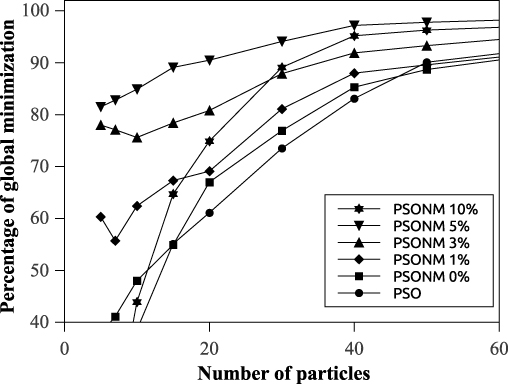
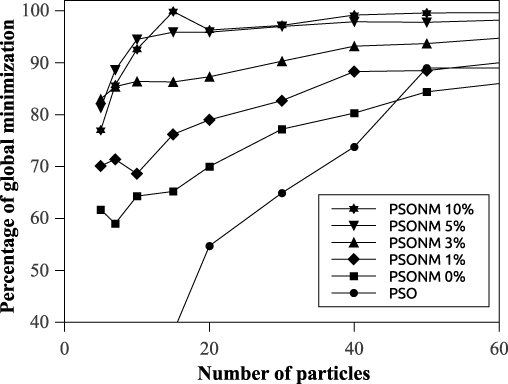
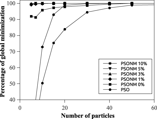
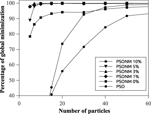
Shown in figures 5, 6, 7 and 8 are the percentages of function minimization with respect to particle numbers, for Ackley’s function (2-D), Griewank function (2-D), Rastrigin function (3-D) and Rastrigin function (4-D), respectively. It can be seen in these figures, as expected, the larger number of particles, the greater the percentage of function minimization, but the particles repositioning presents benefits only for percentages up to 5%, percentages of repositioning greater than 5% leads to poor performance. The large amount of results presented in B makes this clearer, although this is not true for all test functions, in few cases 10% of particles repositioning probability it was obtained best results.
Figure 5.
Percentage of success in minimization of Ackley’s function (2-D). A comparison of PSO and PSO-NM with varying probabilities of repositioning.
Figure 6.
Percentage of success in minimization of Griewank function (2-D). A comparison of PSO and PSO-NM with varying probabilities of repositioning.
Figure 7.
Percentage of success in minimization of Rastrigin function (3-D). A comparison of PSO and PSO-NM with varying probabilities of repositioning.
Figure 8.
Percentage of success in minimization of Rastrigin function (4-D). A comparison of PSO and PSO-NM with varying probabilities of repositioning.
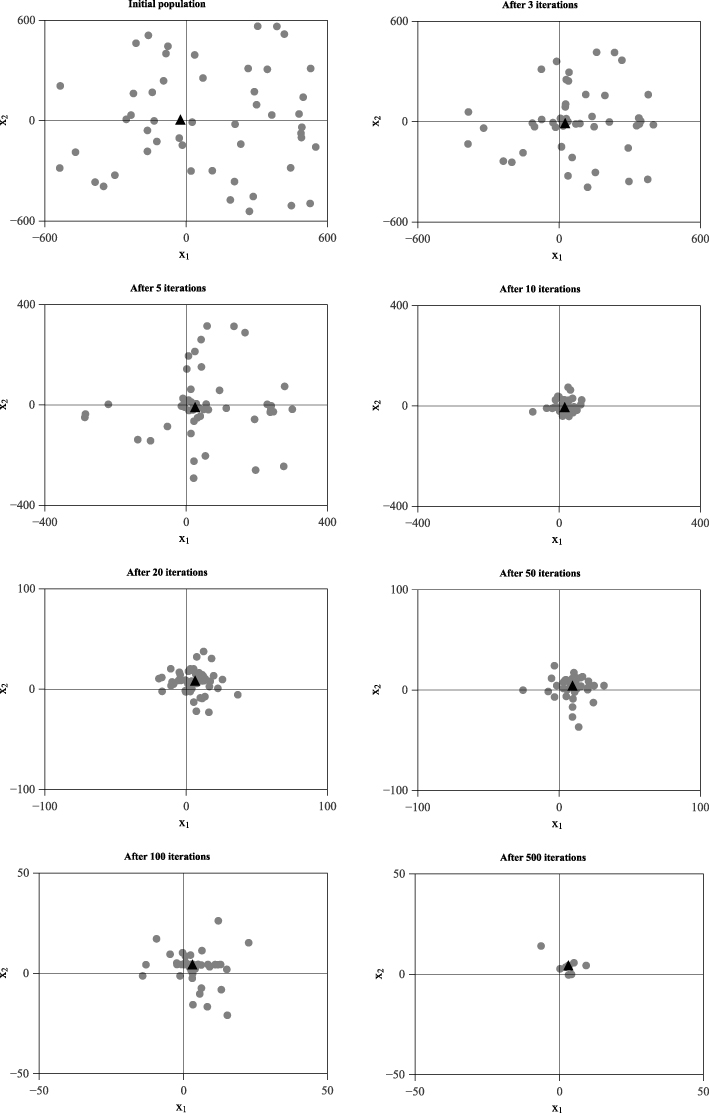
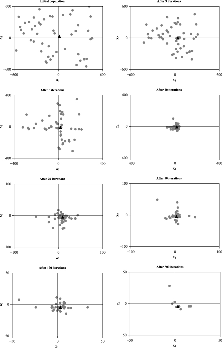
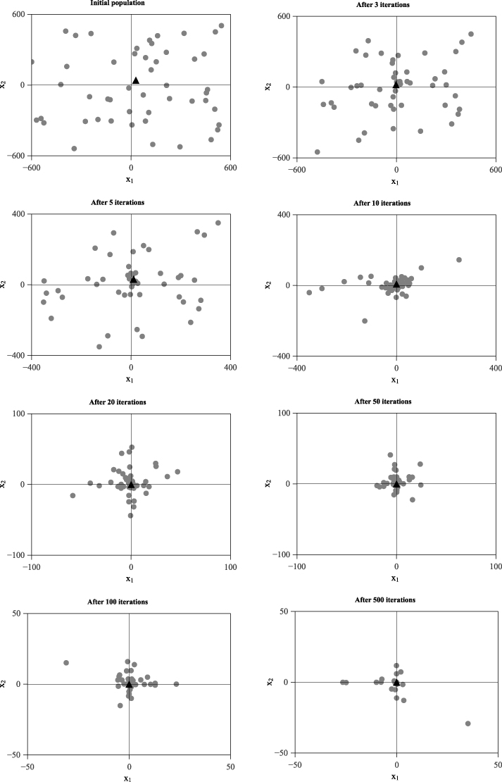
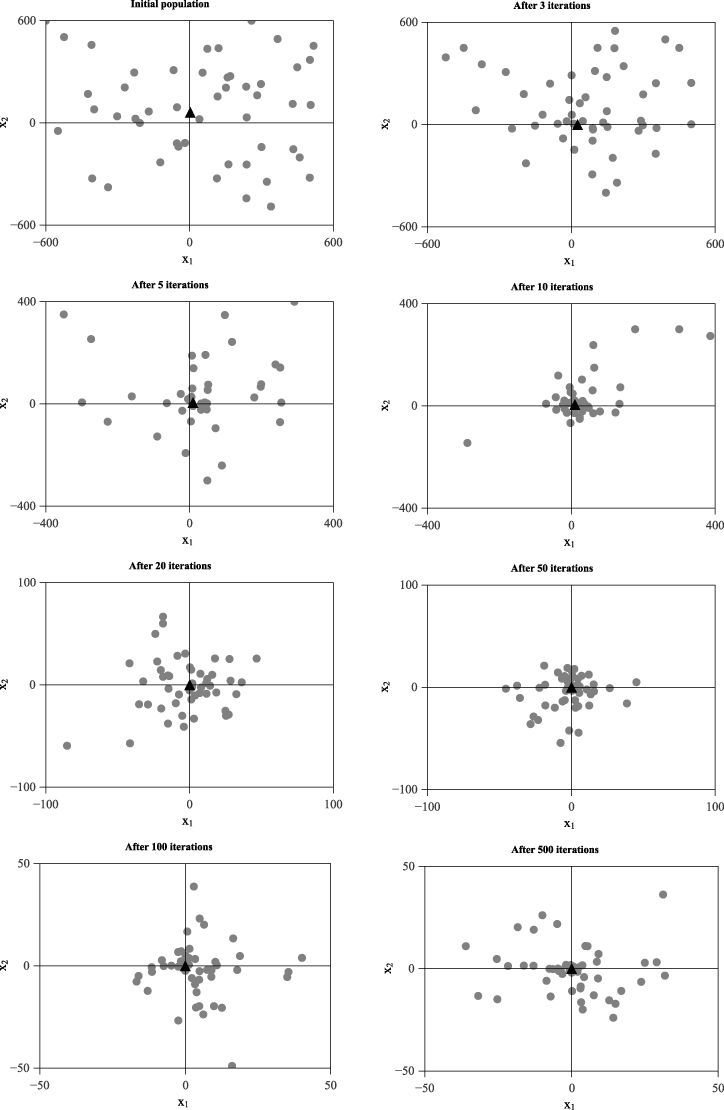
Figures 9, 10, 11 and 12 show the particle positions, in the search region, at some iterations for the PSO and proposed PSO-NM methods, for the Griewank function (2-D), with global minimum at X = (0, 0). In these figures, it is clear that the particle repositioning causes a greater exploration of search region, which explains the reason of the higher percentage of success in obtaining the global minimum. Also, can be seen in figures 9 and 10 the particles getting stuck on a local minimum, and particles stay there, at least until the iteration of number 500, but in the figures 11 and 12, the global best particles move away from the local minimum just after 20 iterations. These facts reinforces the idea that the proposed methods is efficient in avoiding the PSO method of getting stuck in a local minimum, but the repositioning of just the particle with the current global best position is not good enough.
Figure 9.
Particles positions, at some iterations, for PSO method with 50 particles applied to Griewank function (2-D). A black triangle (▴) for current global best and gray circle (∙) for particles.
Figure 10.
Particles positions, at some iterations, for PSO-NM method with 50 particles and 0% of particles repositioning applied to Griewank function (2-D). A black triangle (▴) for current global best and gray circle (∙) for particles.
Figure 11.
Particles positions, at some iterations, for PSO-NM method with 50 particles and 3% of particles repositioning applied to Griewank function (2-D). A black triangle (▴) for current global best and gray circle (∙) for particles.
Figure 12.
Particles positions, at some iterations, for PSO-NM method with 50 particles and 10% of particles repositioning applied to Griewank function (2-D). A black triangle (▴) for current global best and gray circle (∙) for particles.
Figure 13.
Progress, in initial iterations, of mean function values at G best position, for PSO and PSO-NM methods with 50 particles and various probabilities of particles repositioning applied to Griewank function (2-D).
Figure 14.
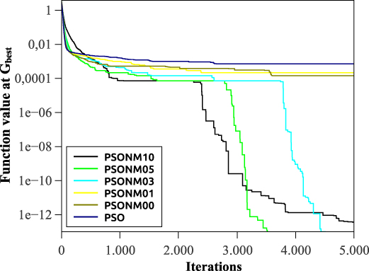
Progress of mean function values at G best position, for PSO and PSO-NM methods with 50 particles and various probabilities of particles repositioning applied to Griewank function (2-D).
Figures 13 and 14 depicts the mean of Griewank function (2-D) value at global best position ever reached. Figure 13 shows the behavior for the first 200 iterations and figure 14 shows the behavior of mean function values until 5000 iterations. Initially, PSO method converges faster than PSO-NM, but analyzing the figure 13, it can be seen that the particles get stuck at a local minimum, and a higher probability of particles repositioning easily to escape from a local minimum. However, using 10% of particles repositioning presented some difficulty on the convergence process even after escaping from the local minimum. Again, it was clear that the proposed PSO-NM method presents advantages, but the percentage of particles repositioning should not be so high.
Conclusions
In this work we studied the effect of adding a step on PSO algorithm regarding to the percentage of success on reaching the global minimum of functions with several local minima. In this new step, the repositioning of the global best and other particles was performed, depending on a repositioning probability, which aims to avoid the global best particle getting stuck in a local minimum. Several simulations were carried out by computational studies, which demonstrated that this new step works very well. The repositioning of particle of global best solution increases the percentage of success on reaching the global best solution, but better results can be obtained applying the repositioning strategy to other particles with repositioning probabilities up to 5%. Repositioning probabilities greater than 5% should be avoided because, in various cases, this presented worse results. The strategy, which we proposed to avoid getting stuck on local optimum is very simple and can be easily adapted to other heuristic optimization methods.
The test functions employed in this work are given below:
Function 1 (2-D): Rosenbrock function
Global optimum at X∗ = (1.0, 1.0) with f (X∗) = 0.0
Function evaluated in the range xi ∈ [−100, 100] ∀ i
Function 2 (2-D): Schaffer function no 2
Global optimum at X∗ = (0.0, 0.0) with f (X∗) = 0.0
Function evaluated in the range xi ∈ [−100, 100] ∀ i
Function 3 (2-D): Schaffer function no 4
Global optimum at X∗ = (0.0, 1.25313) with f (X∗) = 0.292579
Function evaluated in the range xi ∈ [−100, 100] ∀ i
Function 4 (2-D): Eggholder function
Global optimum at X∗ = (512.0, 404.2319) with f (X∗) = −959.6407
Function evaluated in the range xi ∈ [−512, 512] ∀ i
Function 5 (2-D): Hölder table function
Global optimum at X∗ = (±8.05502, ±9.66459) with f (X∗) = −19.2085
Function evaluated in the range xi ∈ [−100, 100] ∀ i
Function 6 (2-D): Ackley’s function
+ e + 20.0
Global optimum at X∗ = (0.0, 0.0) with f (X∗) = 0.0
Function evaluated in the range xi ∈ [−500, 500] ∀ i
Function 7 (2-D): Beale’s function
Global optimum at X∗ = (3.0, 0.5) with f (X∗) = 0.0
Function evaluated in the range xi ∈ [−500, 500] ∀ i
Function 8 (2-D): Goldstein-Price function
Global optimum at X∗ = (0.0, −1.0) with f (X∗) = 3.0
Function evaluated in the range xi ∈ [−500, 500] ∀ i
Global optimum at X∗ = (1.0, 1.0) with f (X∗) = 0.0
Function evaluated in the range xi ∈ [−500, 500] ∀ i
Function 10 (2-D): Six-Hump Camel function
Global optimum at X∗ = ±(0.0898, −0.7126) with f (X∗) = −1.0316
Function evaluated in the range xi ∈ [−500, 500] ∀ i
Function 11 (2-D): Bukin function no 6
Global optimum at X∗ = (−10.0, 1.0) with f (X∗) = 0.0
Function evaluated in the range x1 ∈ [−15, −5] and x2 ∈ [−3, −3]
Function 12 (2-D): Cross-in-Tray
Global optimum at X∗ = (±1.3491, ±1.3491) with f (X∗) = −2.06261
Function evaluated in the range xi ∈ [−100, 100] ∀ i
Function 13 (2-D): Drop Wave function
Global optimum at X∗ = (0.0, 0.0) with f (X∗) = −1.0
Function evaluated in the range xi ∈ [−500, 500] ∀ i
Function 14 (2-D): Rastrigin function
with n = 2
Global optimum at X∗ = (0.0, 0.0) with f (X∗) = 0.0
Function evaluated in the range xi ∈ [−500, 500] ∀ i
Function 15 (2-D): Griewank function
with n = 2
Global optimum at X∗ = (0.0, 0.0) with f (X∗) = 0.0
Function evaluated in the range xi ∈ [−600, 600] ∀ i
Function 16 (2-D): Schwefel function
with n = 2
Global optimum at X∗ = (420.9687, 420.9687) with f (X∗) = 0.0
Function evaluated in the range xi ∈ [−500, 500] ∀ i
Function 17 (3-D): Rastrigin function
with n = 3
Global optimum at X∗ = (0.0, 0.0, 0.0) with f (X∗) = 0.0
Function evaluated in the range xi ∈ [−500, 500] ∀ i
Function 18 (3-D): Griewank function
with n = 3
Global optimum at X∗ = (0.0, 0.0, 0.0) with f (X∗) = 0.0
Function evaluated in the range xi ∈ [−600, 600] ∀ i
Function 19 (3-D): Schwefel function
with n = 3
Global optimum at X∗ = (420.9687, 420.9687, 420.9687) with f (X∗) = 0.0
Function evaluated in the range xi ∈ [−500, 500] ∀ i
Function 20 (4-D): Rosenbrock function
Global optimum at X∗ = (1.0, 1.0, 1.0, 1.0) with f (X∗) = 0.0
Function evaluated in the range xi ∈ [−100, 100] ∀ i
Function 21 (4-D): Wood Function
Global optimum at X∗ = (1.0, 1.0, 1.0, 1.0) with f (X∗) = 0.0
Function evaluated in the range xi ∈ [−100, 100] ∀ i
Function 22 (4-D): Schwefel function
with n = 4
Global optimum at X∗ = (420.9687, 420.9687, 420.9687, 420.9687) with f (X∗) = 0.0
Function evaluated in the range xi ∈ [−500, 500] ∀ i
Function 23 (4-D): Rastrigin function
with n = 4
Global optimum at X∗ = (0.0, 0.0, 0.0, 0.0) with f (X∗) = 0.0
Function evaluated in the range xi ∈ [−500, 500] ∀ i
Function 24 (4-D): Griewank function
with n = 4
Global optimum at X∗ = (0.0, 0.0, 0.0, 0.0) with f (X∗) = 0.0
Function evaluated in the range xi ∈ [−600, 600] ∀ i
The percentage of success on obtaining the global minimum for all test functions employed in this work are given in Tables B.1–B.24.
n
PSO
PSO-NM with probability of repositioning
0%
1%
2%
3%
4%
5%
7%
10%
5
39.9
99.9
100.0
100.0
100.0
99.0
95.7
67.7
18.6
7
100.0
100.0
100.0
100.0
100.0
99.9
99.5
90.1
40.8
10
100.0
100.0
100.0
100.0
100.0
100.0
99.9
98.5
66.9
15
100.0
100.0
100.0
100.0
100.0
100.0
100.0
100.0
90.0
20
100.0
100.0
100.0
100.0
100.0
100.0
100.0
100.0
96.3
30
100.0
100.0
100.0
100.0
100.0
100.0
100.0
100.0
99.1
40
100.0
100.0
100.0
100.0
100.0
100.0
100.0
100.0
99.5
50
100.0
100.0
100.0
100.0
100.0
100.0
100.0
100.0
100.0
100
100.0
100.0
100.0
100.0
100.0
100.0
100.0
100.0
100.0
200
100.0
100.0
100.0
100.0
100.0
100.0
100.0
100.0
100.0
300
100.0
100.0
100.0
100.0
100.0
100.0
100.0
100.0
100.0
500
100.0
100.0
100.0
100.0
100.0
100.0
100.0
100.0
100.0
Table B.1
Percentage of success in minimization of Rosenbrock function (2-D). A comparison of PSO and PSO-NM with varying probabilities of repositioning.
n
PSO
PSO-NM with probability of repositioning
0%
1%
2%
3%
4%
5%
7%
10%
5
92.8
100.0
100.0
100.0
100.0
100.0
100.0
100.0
100.0
7
99.6
100.0
100.0
100.0
100.0
100.0
100.0
100.0
100.0
10
100.0
100.0
100.0
100.0
100.0
100.0
100.0
100.0
100.0
15
100.0
100.0
100.0
100.0
100.0
100.0
100.0
100.0
100.0
20
100.0
100.0
100.0
100.0
100.0
100.0
100.0
100.0
100.0
30
100.0
100.0
100.0
100.0
100.0
100.0
100.0
100.0
100.0
40
100.0
100.0
100.0
100.0
100.0
100.0
100.0
100.0
100.0
50
100.0
100.0
100.0
100.0
100.0
100.0
100.0
100.0
100.0
100
100.0
100.0
100.0
100.0
100.0
100.0
100.0
100.0
100.0
200
100.0
100.0
100.0
100.0
100.0
100.0
100.0
100.0
100.0
300
100.0
100.0
100.0
100.0
100.0
100.0
100.0
100.0
100.0
500
100.0
100.0
100.0
100.0
100.0
100.0
100.0
100.0
100.0
Table B.2
Percentage of success in minimization of Schaffer function no 2 (2-D). A comparison of PSO and PSO-NM with varying probabilities of repositioning.
n
PSO
PSO-NM with probability of repositioning
0%
1%
2%
3%
4%
5%
7%
10%
5
85.4
99.7
99.6
99.4
99.2
99.4
99.2
97.3
89.6
7
98.5
100.0
100.0
99.9
99.6
100.0
99.7
99.4
97.5
10
99.6
100.0
100.0
100.0
100.0
100.0
100.0
100.0
99.4
15
100.0
100.0
100.0
100.0
100.0
100.0
100.0
100.0
99.8
20
100.0
100.0
100.0
100.0
100.0
100.0
100.0
100.0
100.0
30
100.0
100.0
100.0
100.0
100.0
100.0
100.0
100.0
100.0
40
100.0
100.0
100.0
100.0
100.0
100.0
100.0
100.0
100.0
50
100.0
100.0
100.0
100.0
100.0
100.0
100.0
100.0
100.0
100
100.0
100.0
100.0
100.0
100.0
100.0
100.0
100.0
100.0
200
100.0
100.0
100.0
100.0
100.0
100.0
100.0
100.0
100.0
300
100.0
100.0
100.0
100.0
100.0
100.0
100.0
100.0
100.0
500
100.0
100.0
100.0
100.0
100.0
100.0
100.0
100.0
100.0
Table B.3
Percentage of success in minimization of Schaffer function no 3 (2-D). A comparison of PSO and PSO-NM with varying probabilities of repositioning.
n
PSO
PSO-NM with probability of repositioning
0%
1%
2%
3%
4%
5%
7%
10%
5
0.3
1.3
5.6
9.1
15.6
24.3
23.9
22.6
19.0
7
0.3
2.0
5.7
14.0
22.1
36.1
42.5
55.1
53.3
10
0.8
1.9
7.5
15.4
27.2
41.7
55.7
66.0
77.8
15
1.7
2.6
8.7
18.5
27.2
42.4
56.8
78.0
87.5
20
1.4
3.2
12.0
20.2
31.5
44.4
61.2
80.4
91.7
30
2.3
3.2
20.4
28.8
39.1
52.6
64.8
84.2
94.7
40
4.0
5.0
26.9
36.8
48.4
58.9
71.9
88.3
94.8
50
2.8
4.2
31.4
43.6
58.7
69.1
76.3
89.1
97.0
100
4.7
6.0
49.5
66.4
79.2
88.1
94.4
98.4
99.6
200
6.0
7.0
70.2
85.8
95.1
98.2
99.2
99.9
100.0
300
6.5
7.0
84.0
95.2
97.9
99.8
99.9
100.0
100.0
500
9.4
7.8
94.0
98.6
99.6
100.0
100.0
100.0
100.0
Table B.4
Percentage of success in minimization of Eggholder function (2-D). A comparison of PSO and PSO-NM with varying probabilities of repositioning.
n
PSO
PSO-NM with probability of repositioning
0%
1%
2%
3%
4%
5%
7%
10%
5
31.2
57.8
78.9
87.3
92.0
93.4
93.3
93.7
94.2
7
33.5
65.9
84.0
86.8
93.5
96.9
96.7
97.1
98.4
10
51.8
70.4
92.7
94.6
96.4
97.4
99.1
99.1
99.5
15
64.3
76.5
98.3
98.7
99.1
99.3
99.9
99.9
100.0
20
77.6
85.7
99.7
99.8
99.9
99.9
99.9
100.0
100.0
30
89.3
94.8
100.0
100.0
100.0
100.0
100.0
100.0
100.0
40
94.9
96.1
100.0
100.0
100.0
100.0
100.0
100.0
100.0
50
97.5
98.4
100.0
100.0
100.0
100.0
100.0
100.0
100.0
100
99.8
100.0
100.0
100.0
100.0
100.0
100.0
100.0
100.0
200
100.0
100.0
100.0
100.0
100.0
100.0
100.0
100.0
100.0
300
100.0
100.0
100.0
100.0
100.0
100.0
100.0
100.0
100.0
500
100.0
100.0
100.0
100.0
100.0
100.0
100.0
100.0
100.0
Table B.5
Percentage of success in minimization of Hölder table function (2-D). A comparison of PSO and PSO-NM with varying probabilities of repositioning.
n
PSO
PSO-NM with probability of repositioning
0%
1%
2%
3%
4%
5%
7%
10%
5
15.9
37.7
60.3
74.5
78.0
79.5
81.5
56.1
7.9
7
28.1
41.1
55.7
68.8
77.1
81.1
82.8
74.2
20.7
10
38.5
48.0
62.4
66.5
75.6
81.3
84.9
81.0
43.9
15
55.1
54.9
67.3
73.2
78.4
83.8
89.1
89.2
64.7
20
61.1
67.0
69.1
75.7
80.8
84.6
90.5
94.7
74.9
30
73.5
76.9
81.1
85.3
87.9
91.2
94.1
97.4
89.1
40
83.1
85.3
88.0
87.1
91.9
94.2
97.2
99.3
95.2
50
90.1
88.7
89.6
92.5
93.3
97.4
97.8
99.8
96.3
100
98.5
98.0
97.1
98.8
99.3
99.9
99.9
100.0
99.1
200
100.0
100.0
100.0
99.8
100.0
100.0
100.0
100.0
100.0
300
100.0
100.0
100.0
100.0
100.0
100.0
100.0
100.0
100.0
500
100.0
100.0
100.0
100.0
100.0
100.0
100.0
100.0
100.0
Table B.6
Percentage of success in minimization of Ackley’s function (2-D). A comparison of PSO and PSO-NM with varying probabilities of repositioning.
n
PSO
PSO-NM with probability of repositioning
0%
1%
2%
3%
4%
5%
7%
10%
5
30.7
66.6
69.6
70.6
68.5
67.6
66.6
72.5
74.0
7
64.6
69.7
70.8
72.3
76.2
74.9
70.6
73.9
74.5
10
70.4
71.3
72.1
73.3
83.6
82.9
81.1
77.7
77.3
15
79.5
77.8
76.4
80.6
84.3
88.4
90.6
89.2
83.8
20
82.0
83.0
82.7
84.0
87.4
91.9
93.7
94.0
89.8
30
83.5
88.2
89.2
88.3
89.6
94.1
96.3
98.4
96.1
40
90.2
89.8
89.4
90.4
94.0
95.6
98.5
99.3
98.7
50
92.9
93.3
94.2
95.1
94.6
96.4
98.1
99.9
99.7
100
97.8
98.9
98.6
99.0
98.7
99.1
99.7
100.0
100.0
200
99.7
99.9
99.7
100.0
100.0
100.0
100.0
100.0
100.0
300
100.0
100.0
100.0
100.0
100.0
100.0
100.0
100.0
100.0
500
100.0
100.0
100.0
100.0
100.0
100.0
100.0
100.0
100.0
Table B.7
Percentage of success in minimization of Beale’s function (2-D). A comparison of PSO and PSO-NM with varying probabilities of repositioning.
n
PSO
PSO-NM with probability of repositioning
0%
1%
2%
3%
4%
5%
7%
10%
5
17.6
93.3
98.5
98.0
98.8
98.7
99.6
99.2
77.3
7
47.1
97.8
99.6
99.3
98.7
99.5
99.9
99.7
94.6
10
78.0
99.5
100.0
99.8
99.8
100.0
99.9
100.0
99.8
15
98.0
99.9
100.0
100.0
100.0
100.0
100.0
100.0
99.2
20
99.9
100.0
100.0
100.0
100.0
100.0
100.0
100.0
99.2
30
100.0
100.0
100.0
100.0
100.0
100.0
100.0
100.0
99.9
40
100.0
100.0
100.0
100.0
100.0
100.0
100.0
100.0
99.8
50
100.0
100.0
100.0
100.0
100.0
100.0
100.0
100.0
100.0
100
100.0
100.0
100.0
100.0
100.0
100.0
100.0
100.0
100.0
200
100.0
100.0
100.0
100.0
100.0
100.0
100.0
100.0
100.0
300
100.0
100.0
100.0
100.0
100.0
100.0
100.0
100.0
100.0
500
100.0
100.0
100.0
100.0
100.0
100.0
100.0
100.0
100.0
Table B.8
Percentage of success in minimization of Goldstein-Price function (2-D). A comparison of PSO and PSO-NM with varying probabilities of repositioning.
n
PSO
PSO-NM with probability of repositioning
0%
1%
2%
3%
4%
5%
7%
10%
5
81.8
100.0
100.0
100.0
100.0
100.0
100.0
100.0
99.4
7
97.3
100.0
100.0
100.0
100.0
100.0
100.0
100.0
99.8
10
99.8
100.0
100.0
100.0
100.0
100.0
100.0
100.0
100.0
15
100.0
100.0
100.0
100.0
100.0
100.0
100.0
100.0
99.8
20
100.0
100.0
100.0
100.0
100.0
100.0
100.0
100.0
99.9
30
100.0
100.0
100.0
100.0
100.0
100.0
100.0
100.0
100.0
40
100.0
100.0
100.0
100.0
100.0
100.0
100.0
100.0
100.0
50
100.0
100.0
100.0
100.0
100.0
100.0
100.0
100.0
100.0
100
100.0
100.0
100.0
100.0
100.0
100.0
100.0
100.0
100.0
200
100.0
100.0
100.0
100.0
100.0
100.0
100.0
100.0
100.0
300
100.0
100.0
100.0
100.0
100.0
100.0
100.0
100.0
100.0
500
100.0
100.0
100.0
100.0
100.0
100.0
100.0
100.0
100.0
Table B.9
Percentage of success in minimization of Levy function no 13 (2-D). A comparison of PSO and PSO-NM with varying probabilities of repositioning.
n
PSO
PSO-NM with probability of repositioning
0%
1%
2%
3%
4%
5%
7%
10%
5
74.5
100.0
100.0
100.0
99.9
100.0
99.8
99.7
97.8
7
97.8
100.0
100.0
100.0
100.0
100.0
100.0
100.0
100.0
10
99.9
100.0
100.0
100.0
100.0
100.0
100.0
100.0
100.0
15
100.0
100.0
100.0
100.0
100.0
100.0
100.0
100.0
99.7
20
100.0
100.0
100.0
100.0
100.0
100.0
100.0
100.0
100.0
30
100.0
100.0
100.0
100.0
100.0
100.0
100.0
100.0
100.0
40
100.0
100.0
100.0
100.0
100.0
100.0
100.0
100.0
100.0
50
100.0
100.0
100.0
100.0
100.0
100.0
100.0
100.0
100.0
100
100.0
100.0
100.0
100.0
100.0
100.0
100.0
100.0
100.0
200
100.0
100.0
100.0
100.0
100.0
100.0
100.0
100.0
100.0
300
100.0
100.0
100.0
100.0
100.0
100.0
100.0
100.0
100.0
500
100.0
100.0
100.0
100.0
100.0
100.0
100.0
100.0
100.0
Table B.10
Percentage of success in minimization of Six-Hump Camel function (2-D). A comparison of PSO and PSO-NM with varying probabilities of repositioning.
n
PSO
PSO-NM with probability of repositioning
0%
1%
2%
3%
4%
5%
7%
10%
5
0.4
3.7
2.7
5.5
4.7
5.8
8.6
10.0
13.8
7
0.5
1.3
2.1
3.8
5.0
6.8
7.0
11.0
12.1
10
0.4
2.0
1.8
3.1
5.0
6.4
5.5
11.3
14.7
15
0.4
1.2
2.2
2.4
4.1
6.2
5.2
10.7
14.8
20
0.7
0.9
1.3
2.1
3.4
6.3
8.3
10.8
14.7
30
0.7
0.7
1.4
2.3
2.7
5.4
6.7
10.2
14.8
40
0.8
0.3
0.7
1.0
2.8
5.3
4.9
9.1
14.7
50
0.7
0.5
1.1
1.7
3.0
4.0
5.8
10.5
12.1
100
0.5
0.7
1.6
1.5
2.1
4.0
7.2
9.1
14.1
200
0.6
0.4
0.7
2.1
2.6
4.0
5.1
9.7
14.7
300
0.6
0.2
0.6
1.2
2.5
4.7
5.8
10.8
15.6
500
0.7
0.9
1.2
1.6
2.2
5.0
6.7
10.5
15.3
Table B.11
Percentage of success in minimization of Bukin function (2-D). A comparison of PSO and PSO-NM with varying probabilities of repositioning.
n
PSO
PSO-NM with probability of repositioning
0%
1%
2%
3%
4%
5%
7%
10%
5
96.9
100.0
100.0
100.0
100.0
100.0
100.0
100.0
100.0
7
99.9
100.0
100.0
100.0
100.0
100.0
100.0
100.0
100.0
10
100.0
100.0
100.0
100.0
100.0
100.0
100.0
100.0
100.0
15
100.0
100.0
100.0
100.0
100.0
100.0
100.0
100.0
100.0
20
100.0
100.0
100.0
100.0
100.0
100.0
100.0
100.0
100.0
30
100.0
100.0
100.0
100.0
100.0
100.0
100.0
100.0
100.0
40
100.0
100.0
100.0
100.0
100.0
100.0
100.0
100.0
100.0
50
100.0
100.0
100.0
100.0
100.0
100.0
100.0
100.0
100.0
100
100.0
100.0
100.0
100.0
100.0
100.0
100.0
100.0
100.0
200
100.0
100.0
100.0
100.0
100.0
100.0
100.0
100.0
100.0
300
100.0
100.0
100.0
100.0
100.0
100.0
100.0
100.0
100.0
500
100.0
100.0
100.0
100.0
100.0
100.0
100.0
100.0
100.0
Table B.12
Percentage of success in minimization of Cros-in-Tray function (2-D). A comparison of PSO and PSO-NM with varying probabilities of repositioning.
n
PSO
PSO-NM with probability of repositioning
0%
1%
2%
3%
4%
5%
7%
10%
5
31.0
69.2
86.2
90.5
91.2
90.9
91.0
91.9
80.6
7
51.9
74.8
91.7
95.2
96.6
96.3
96.7
97.3
95.9
10
66.8
85.2
94.4
97.4
99.0
99.1
99.4
99.5
99.1
15
82.1
90.7
97.0
99.2
99.7
99.8
100.0
99.9
99.0
20
87.7
96.1
99.0
100.0
100.0
100.0
99.9
100.0
98.9
30
95.5
98.7
99.9
99.9
100.0
100.0
100.0
100.0
99.5
40
98.9
99.8
100.0
100.0
100.0
100.0
100.0
100.0
100.0
50
99.6
99.8
99.9
100.0
100.0
100.0
100.0
100.0
100.0
100
100.0
100.0
100.0
100.0
100.0
100.0
100.0
100.0
100.0
200
100.0
100.0
100.0
100.0
100.0
100.0
100.0
100.0
100.0
300
100.0
100.0
100.0
100.0
100.0
100.0
100.0
100.0
100.0
500
100.0
100.0
100.0
100.0
100.0
100.0
100.0
100.0
100.0
Table B.13
Percentage of success in minimization of Drop Wave function (2-D). A comparison of PSO and PSO-NM with varying probabilities of repositioning.
n
PSO
PSO-NM with probability of repositioning
0%
1%
2%
3%
4%
5%
7%
10%
5
42.2
98.9
99.9
100.0
99.9
100.0
100.0
100.0
84.8
7
69.1
99.2
100.0
100.0
100.0
100.0
100.0
100.0
96.8
10
86.8
99.6
100.0
100.0
100.0
100.0
100.0
100.0
99.5
15
96.1
100.0
100.0
100.0
100.0
100.0
100.0
100.0
99.9
20
98.3
99.8
100.0
100.0
100.0
100.0
100.0
100.0
99.8
30
100.0
100.0
100.0
100.0
100.0
100.0
100.0
100.0
100.0
40
100.0
100.0
100.0
100.0
100.0
100.0
100.0
100.0
100.0
50
100.0
100.0
100.0
100.0
100.0
100.0
100.0
100.0
100.0
100
100.0
100.0
100.0
100.0
100.0
100.0
100.0
100.0
100.0
200
100.0
100.0
100.0
100.0
100.0
100.0
100.0
100.0
100.0
300
100.0
100.0
100.0
100.0
100.0
100.0
100.0
100.0
100.0
500
100.0
100.0
100.0
100.0
100.0
100.0
100.0
100.0
100.0
Table B.14
Percentage of success in minimization of Rastrigin function (2-D). A comparison of PSO and PSO-NM with varying probabilities of repositioning.
n
PSO
PSO-NM with probability of repositioning
0%
1%
2%
3%
4%
5%
7%
10%
5
3.9
61.7
70.1
80.1
83.0
81.1
81.3
78.9
77.0
7
8.9
59.0
71.4
80.6
85.4
90.9
88.6
88.7
85.7
10
21.3
64.3
68.6
80.0
86.4
93.0
94.5
93.3
92.6
15
38.0
65.2
76.2
82.6
86.3
92.1
95.9
97.2
99.9
20
54.7
70.0
79.0
82.6
87.3
93.4
95.9
97.3
96.3
30
64.9
77.2
82.7
86.6
90.3
94.6
97.0
99.5
97.2
40
73.8
80.3
88.3
91.2
93.2
96.7
97.9
99.7
99.2
50
89.0
84.4
88.5
92.5
93.7
97.0
97.8
99.9
99.6
100
89.0
92.5
96.1
97.4
98.9
99.3
99.9
100.0
100.0
200
95.6
96.5
98.9
99.7
100.0
100.0
100.0
100.0
100.0
300
97.5
98.0
100.0
100.0
100.0
99.9
100.0
100.0
100.0
500
99.2
99.8
99.9
100.0
100.0
100.0
100.0
100.0
100.0
Table B.15
Percentage of success in minimization of Griewank function (2-D). A comparison of PSO and PSO-NM with varying probabilities of repositioning.
n
PSO
PSO-NM with probability of repositioning
0%
1%
2%
3%
4%
5%
7%
10%
5
5.8
8.3
20.5
48.8
58.4
64.8
67.8
69.4
44.0
7
10.0
9.3
22.4
49.7
70.9
77.0
81.4
85.2
83.6
10
16.6
14.4
29.3
48.9
74.0
85.6
90.8
93.6
97.5
15
24.8
20.2
38.1
52.4
77.0
89.9
97.0
98.3
99.6
20
29.8
27.3
47.7
61.9
81.3
94.5
97.5
99.3
100.0
30
45.5
36.5
58.6
78.1
91.3
97.0
99.5
100.0
100.0
40
52.2
43.9
74.5
90.2
96.7
98.9
99.9
100.0
100.0
50
62.2
52.5
85.2
94.7
98.2
100.0
100.0
100.0
100.0
100
82.6
77.3
97.4
99.9
100.0
100.0
100.0
100.0
100.0
200
97.2
96.4
100.0
100.0
100.0
100.0
100.0
100.0
100.0
300
99.9
99.4
100.0
100.0
100.0
100.0
100.0
100.0
100.0
500
100.0
99.8
100.0
100.0
100.0
100.0
100.0
100.0
100.0
Table B.16
Percentage of success in minimization of Schwefel function (2-D). A comparison of PSO and PSO-NM with varying probabilities of repositioning.
n
PSO
PSO-NM with probability of repositioning
0%
1%
2%
3%
4%
5%
7%
10%
5
5.9
92.0
99.2
100.0
99.9
99.9
99.3
84.9
14.2
7
25.2
91.3
99.6
99.9
100.0
100.0
100.0
96.9
39.5
10
50.4
95.8
99.8
100.0
100.0
100.0
100.0
99.8
72.9
15
75.4
97.3
100.0
100.0
100.0
100.0
100.0
100.0
93.0
20
83.9
97.9
100.0
100.0
100.0
100.0
100.0
100.0
98.8
30
94.5
98.7
100.0
100.0
100.0
100.0
100.0
100.0
99.8
40
97.2
99.5
100.0
100.0
100.0
100.0
100.0
100.0
99.9
50
98.9
100.0
100.0
100.0
100.0
100.0
100.0
100.0
100.0
100
99.9
100.0
100.0
100.0
100.0
100.0
100.0
100.0
100.0
200
100.0
100.0
100.0
100.0
100.0
100.0
100.0
100.0
100.0
300
100.0
100.0
100.0
100.0
100.0
100.0
100.0
100.0
100.0
500
100.0
100.0
100.0
100.0
100.0
100.0
100.0
100.0
100.0
Table B.17
Percentage of success in minimization of Rastrigin function (3-D). A comparison of PSO and PSO-NM with varying probabilities of repositioning.
n
PSO
PSO-NM with probability of repositioning
0%
1%
2%
3%
4%
5%
7%
10%
5
0.0
13.1
16.5
19.7
20.8
20.7
15.3
13.7
10.8
7
0.4
11.3
17.4
20.9
25.8
26.0
20.3
23.1
19.2
10
1.2
11.4
14.9
22.7
29.2
34.7
32.9
29.9
27.5
15
3.4
15.7
20.2
26.9
33.7
44.1
42.5
38.4
39.6
20
11.1
14.5
21.6
27.8
38.5
45.6
49.4
50.7
49.4
30
16.3
22.9
28.7
33.5
43.7
49.2
56.3
61.0
58.1
40
25.5
31.5
32.4
37.6
46.0
53.6
60.3
66.7
67.8
50
30.9
34.0
39.3
45.3
49.2
59.6
64.8
76.2
74.3
100
50.3
54.2
59.0
60.4
64.6
72.4
80.5
88.2
91.0
200
67.4
71.2
70.0
77.6
80.3
85.3
90.5
97.8
99.1
300
77.9
79.9
83.2
87.1
89.8
93.6
95.8
99.2
99.4
500
87.0
89.9
92.9
93.9
96.0
98.0
98.1
99.9
100.0
Table B.18
Percentage of success in minimization of Griewank function (3-D). A comparison of PSO and PSO-NM with varying probabilities of repositioning.
n
PSO
PSO-NM with probability of repositioning
0%
1%
2%
3%
4%
5%
7%
10%
5
1.0
1.7
1.8
3.2
4.4
7.5
6.7
3.9
0.0
7
1.4
2.0
2.5
4.3
12.9
27.6
40.3
45.7
17.3
10
2.4
2.8
3.6
6.0
13.5
25.8
49.7
67.2
59.1
15
4.7
3.8
6.3
5.9
14.8
27.4
46.4
78.7
89.2
20
6.2
4.7
7.4
11.7
20.6
33.3
50.4
84.1
95.0
30
8.3
5.9
10.8
21.4
27.2
43.6
60.8
91.1
98.9
40
9.7
8.1
14.7
27.7
39.7
55.3
70.4
93.6
99.6
50
17.4
8.2
19.4
32.9
47.6
64.7
78.4
95.8
99.9
100
26.7
16.2
41.3
62.5
78.6
91.4
96.2
99.7
100.0
200
45.3
31.4
71.8
87.5
98.2
99.6
99.9
100.0
100.0
300
59.1
46.4
86.1
97.6
99.8
100.0
100.0
100.0
100.0
500
76.7
65.2
96.6
99.8
100.0
100.0
100.0
100.0
100.0
Table B.19
Percentage of success in minimization of Schwefel function (3-D). A comparison of PSO and PSO-NM with varying probabilities of repositioning.
n
PSO
PSO-NM with probability of repositioning
0%
1%
2%
3%
4%
5%
7%
10%
5
1.4
92.5
83.1
63.3
26.5
1.9
0.2
0.0
0.0
7
93.0
96.6
92.6
83.3
53.5
14.1
1.7
0.0
0.0
10
99.0
98.2
97.1
90.7
75.5
38.4
8.5
0.1
0.0
15
99.7
99.5
98.9
97.3
91.8
66.1
32.1
1.3
0.0
20
99.8
99.9
99.4
98.6
96.3
85.7
56.3
3.2
0.0
30
100.0
100.0
100.0
100.0
99.2
95.0
80.0
11.6
0.2
40
100.0
100.0
100.0
99.7
99.6
98.7
91.7
25.2
0.2
50
100.0
100.0
99.9
99.9
100.0
99.6
93.9
41.5
0.3
100
100.0
100.0
100.0
100.0
100.0
99.9
99.5
85.6
6.2
200
100.0
100.0
100.0
100.0
100.0
100.0
100.0
98.4
27.0
300
100.0
100.0
100.0
100.0
100.0
100.0
100.0
100.0
56.0
500
100.0
100.0
100.0
100.0
100.0
100.0
100.0
100.0
83.6
Table B.20
Percentage of success in minimization of Rosenbrock function (4-D). A comparison of PSO and PSO-NM with varying probabilities of repositioning.
n
PSO
PSO-NM with probability of repositioning
0%
1%
2%
3%
4%
5%
7%
10%
5
0.1
99.4
98.3
93.2
56.2
4.8
1.3
0.0
0.0
7
85.2
99.8
98.8
97.2
83.5
31.6
3.8
0.2
0.0
10
99.9
99.9
99.4
97.8
93.6
68.6
19.1
1.0
0.1
15
99.7
99.9
99.8
98.8
98.0
90.2
57.8
2.7
0.1
20
100.0
99.9
99.8
99.4
99.3
96.1
82.0
9.2
0.8
30
100.0
100.0
100.0
99.8
99.8
99.6
95.0
32.4
1.2
40
100.0
100.0
100.0
99.9
99.9
99.9
98.9
58.5
3.5
50
100.0
100.0
100.0
100.0
100.0
100.0
99.5
76.6
4.0
100
100.0
100.0
100.0
100.0
100.0
100.0
100.0
99.1
25.2
200
100.0
100.0
100.0
100.0
100.0
100.0
100.0
100.0
73.7
300
100.0
100.0
100.0
100.0
100.0
100.0
100.0
100.0
91.9
500
100.0
100.0
100.0
100.0
100.0
100.0
100.0
100.0
99.5
Table B.21
Percentage of success in minimization of Wood function (4-D). A comparison of PSO and PSO-NM with varying probabilities of repositioning.
n
PSO
PSO-NM with probability of repositioning
0%
1%
2%
3%
4%
5%
7%
10%
5
0.0
0.2
0.4
0.2
0.5
0.5
0.3
0.0
0.0
7
0.1
0.1
0.7
0.3
0.4
0.9
1.1
2.2
0.5
10
0.1
0.5
0.2
1.2
1.0
1.6
2.2
9.5
20.6
15
1.2
0.3
0.7
1.5
2.1
2.5
3.5
11.0
41.6
20
1.6
0.9
1.0
1.2
3.0
3.7
5.1
14.2
50.0
30
1.0
0.8
1.9
2.7
4.0
7.1
10.0
23.7
58.9
40
2.8
1.1
2.0
2.6
5.9
10.2
16.6
30.9
68.5
50
2.4
1.0
2.2
4.1
6.5
11.3
20.1
36.4
76.5
100
3.5
2.1
5.3
10.4
20.3
31.7
44.8
76.2
96.1
200
7.9
4.5
12.8
26.9
48.9
67.9
82.4
96.6
100.0
300
14.4
8.8
22.2
46.5
68.0
84.3
94.5
99.6
100.0
500
20.3
10.6
39.5
69.2
87.4
97.6
99.6
100.0
100.0
Table B.22
Percentage of success in minimization of Schwefel function (4-D). A comparison of PSO and PSO-NM with varying probabilities of repositioning.
n
PSO
PSO-NM with probability of repositioning
0%
1%
2%
3%
4%
5%
7%
10%
5
0.0
0.8
0.5
1.4
1.7
1.4
1.5
1.7
0.7
7
0.2
1.0
1.6
3.8
3.0
2.2
2.4
1.6
1.1
10
0.0
0.9
2.8
4.1
6.8
4.6
5.7
3.8
1.6
15
0.1
2.5
3.6
6.9
11.5
11.0
10.3
6.3
4.5
20
0.7
2.8
3.7
7.5
10.9
15.8
14.4
11.0
8.0
30
2.3
4.2
6.3
9.1
13.3
18.2
19.9
15.6
13.1
40
3.1
5.1
7.8
11.6
16.1
19.6
28.1
22.4
17.5
50
5.5
6.8
13.9
13.4
17.7
23.8
27.0
27.4
22.1
100
15.6
16.6
19.2
21.2
25.3
30.9
39.1
42.6
37.0
200
29.9
29.8
33.8
36.6
39.2
44.2
55.0
66.1
62.2
300
39.5
36.6
39.7
45.7
49.5
55.7
62.6
78.8
71.8
500
54.2
54.0
57.3
59.0
61.9
68.1
76.0
91.9
86.9
Table B.23
Percentage of success in minimization of Griewank function (4-D). A comparison of PSO and PSO-NM with varying probabilities of repositioning.
n
PSO
PSO-NM with probability of repositioning
0%
1%
2%
3%
4%
5%
7%
10%
5
0.3
78.5
97.8
98.9
98.2
96.2
89.0
35.3
0.5
7
7.0
86.3
98.8
99.9
99.9
99.5
97.8
74.7
3.4
10
21.9
90.7
99.4
100.0
100.0
99.9
99.8
95.1
14.3
15
40.8
93.3
99.7
100.0
100.0
100.0
100.0
99.4
45.4
20
55.9
94.2
99.9
100.0
100.0
100.0
100.0
100.0
73.7
30
71.7
94.1
99.7
100.0
100.0
100.0
100.0
100.0
92.7
40
84.4
96.2
99.8
100.0
100.0
100.0
100.0
100.0
97.4
50
91.8
97.3
99.8
100.0
100.0
100.0
100.0
100.0
98.9
100
98.7
99.7
100.0
100.0
100.0
100.0
100.0
100.0
100.0
200
100.0
100.0
100.0
100.0
100.0
100.0
100.0
100.0
100.0
300
100.0
100.0
100.0
100.0
100.0
100.0
100.0
100.0
100.0
500
100.0
100.0
100.0
100.0
100.0
100.0
100.0
100.0
100.0
Table B.24
Percentage of success in minimization of Rastrigin function (4-D). A comparison of PSO and PSO-NM with varying probabilities of repositioning.
Conflict of interest
The authors declare no conflicts of interest.
Acknowledgement
The author would like to thank Marcel Joly for his comments, which helped in the construction of this method and improved the quality of this work.
References
1.
Foroughi NematollahiA, RahiminejadA, VahidiB. A novel physical based meta-heuristic optimization method known as Lightning Attachment Procedure Optimization. Appl Soft Comput. 2017 Oct;59: 596–621.
2.
OkamotoT, HirataH. Global optimization using a multipoint type quasi-chaotic optimization method. Appl Soft Comput. 2013 Feb;13(2):1247–1264.
3.
KirkpatrickS, GelattCDJr, VecchiMP. Optimization by simulated annealing. Science. 1983;220(4598):671–680.
4.
StornR, PriceK. Differential evolution – a simple and efficient heuristic for global optimization over continuous spaces. J Glob Optim. 1997;11(4):341–359.
5.
AlatasB. ACROA: Artificial Chemical Reaction Optimization Algorithm for global optimization. Expert Syst Appl. 2011 Sep;38(10):13170–13180.
6.
KavehA. Water evaporation optimization algorithm. In: Advances in metaheuristic algorithms for optimal design of structures. Cham: Springer International Publishing; 2017. p. 489–509.
HatamlouA. Black hole: a new heuristic optimization approach for data clustering. Inf Sci. 2013 Feb;222: 175–184.
10.
KennedyJ, EberhartR. Particle swarm optimization. In: Proceedings of International Conference on Neural Networks. vol. 4, 1995. p. 1942–1948.
11.
Pacheco da LuzEF, BecceneriJC, de Campos VelhoHF. A new multi-particle collision algorithm for optimization in a high performance environment. J Comput Interdiscip Sci. 2008;1(1):3–10.
12.
YangX-S. Firefly algorithms for multimodal optimization. Lecture Notes in Computer Science (including subseries Lecture Notes in Artificial Intelligence and Lecture Notes in Bioinformatics), LNCS, vol. 5792, Berlin, Heidelberg: Springer; 2009. p. 169–178.
13.
AskarzadehA. A novel metaheuristic method for solving constrained engineering optimization problems: Crow search algorithm. Comput Struct. 2016 Jun;169: 1–12.
14.
MirjaliliS, LewisA. The whale optimization algorithm. Adv Eng Softw. 2016 May;95: 51–67.
15.
MucherinoA, SerefO, SerefO, Erhun KundakciogluO, PardalosP. Monkey search: a novel metaheuristic search for global optimization. In: AIP Conference Proceedings, AIP. vol. 953, Melville, NY: AIP Publishing; 2007. p. 162–173.
16.
YangXS. A new metaheuristic Bat-inspired Algorithm. Studies in Computational Intelligence, vol. 284, Berlin, Heidelberg: Springer; 2010. p. 65–74.
17.
KarabogaD, BasturkB. A powerful and efficient algorithm for numerical function optimization: artificial bee colony (ABC) algorithm. J Glob Optim. 2007 Oct;39(3):459–471.
18.
MirjaliliS, MirjaliliSM, LewisA. Grey wolf optimizer. Adv Eng Softw. 2014 Mar;69: 46–61.
19.
PanW-T. A new fruit fly optimization algorithm: taking the financial distress model as an example. Knowl Based Syst. 2012 Feb;26: 69–74.
20.
MirjaliliS. Dragonfly algorithm: a new meta-heuristic optimization technique for solving single-objective, discrete, and multi-objective problems. Neural Comput Appl. 2016 May;27(4):1053–1073.
21.
CuevasE, CienfuegosM. A new algorithm inspired in the behavior of the social-spider for constrained optimization. Expert Syst Appl. 2014 Feb;41(2):412–425.
YazdaniM, JolaiF. Lion optimization algorithm (LOA): a nature-inspired metaheuristic algorithm. J Comput Des Eng. 2016 Jan;3(1):24–36.
24.
GloverF. Tabu Search—Part I. ORSA J Comput. 1989 Aug;1(3):190–206.
25.
GloverF. Tabu Search—Part II. ORSA J Comput. 1990 Feb;2(1):4–32.
26.
Husseinzadeh KashanA. League championship algorithm (LCA): an algorithm for global optimization inspired by sport championships. Appl Soft Comput. 2014 Mar;16: 171–200.
27.
MoosavianN, Kasaee RoodsariB. Soccer league competition algorithm: a novel meta-heuristic algorithm for optimal design of water distribution networks. Swarm Evol Comput. 2014 Aug;17: 14–24.
28.
TanY, ZhuY. Fireworks algorithm for optimization. Lecture Notes in Computer Science (including subseries Lecture Notes in Artificial Intelligence and Lecture Notes in Bioinformatics), LNCS, vol. 6145, Berlin, Heidelberg: Springer; 2010. p. 355–364.
29.
KavehA, MahdaviVR. Colliding bodies optimization method for optimum design of truss structures with continuous variables. Adv Eng Softw. 2014 Apr;70: 1–12.
30.
KavehA. Tug of war optimization. Advances in Metaheuristic Algorithms for Optimal Design of Structures, Cham: Springer International Publishing; 2017. p. 451–487.
31.
KavehA, DadrasA. A novel meta-heuristic optimization algorithm: thermal exchange optimization. Adv Eng Softw. 2017 Aug;110: 69–84.
YapiciH, CetinkayaN. A new meta-heuristic optimizer: pathfinder algorithm. Appl Soft Comput J. 2019 May;78: 545–568.
34.
HayyolalamV, KazemAAP. Black widow optimization algorithm: a novel meta-heuristic approach for solving engineering optimization problems. Eng Appl Artif Intell. 2020 Jan;87: 103249.
35.
GhasemiM, DavoudkhaniIF, AkbariE, RahimnejadA, GhavidelS, LiL. A novel and effective optimization algorithm for global optimization and its engineering applications: Turbulent Flow of Water-based Optimization (TFWO). Eng Appl Artif Intell. 2020 Jun;92: 103666.
36.
HeidariAA, PahlavaniP. An efficient modified grey wolf optimizer with Lévy flight for optimization tasks. Appl Soft Comput. 2017 Nov;60: 115–134.
37.
YılmazS, Küçüksille EcirU. A new modification approach on bat algorithm for solving optimization problems. Appl Soft Comput. 2015 Mar;28: 259–275.
38.
BeheshtiZ, ShamsuddinSM. Non-parametric particle swarm optimization for global optimization. Appl Soft Comput. 2015 Mar;28: 345–359.
YanB, ZhaoZ, ZhouY, YuanW, LiJ, WuJ, ChengD. A particle swarm optimization algorithm with random learning mechanism and Levy flight for optimization of atomic clusters. Comput Phys Commun. 2017 Oct;219: 79–86.
41.
YanJ, HeW, JiangX, ZhangZ. A novel phase performance evaluation method for particle swarm optimization algorithms using velocity-based state estimation. Appl Soft Comput. 2017 Aug;57: 517–525.
42.
KiranMS. Particle swarm optimization with a new update mechanism. Appl Soft Comput. 2017 Nov;60: 670–678.
43.
ChenY, LiL, PengH, XiaoJ, YangY, ShiY. Particle swarm optimizer with two differential mutation. Appl Soft Comput J. 2017 Dec;61: 314–330.
44.
YelghiA, KöseC. A modified firefly algorithm for global minimum optimization. Appl Soft Comput. 2018 Jan;62: 29–44.
45.
MengT, PanQ-K. An improved fruit fly optimization algorithm for solving the multidimensional knapsack problem. Appl Soft Comput. 2017 Jan;50: 79–93.
46.
WanY, WangM, YeZ, LaiX. A feature selection method based on modified binary coded ant colony optimization algorithm. Appl Soft Comput. 2016 Dec;49: 248–258.
47.
KarabogaD, AkayB. A modified artificial bee colony (ABC) algorithm for constrained optimization problems. Appl Soft Comput. 2011 Apr;11(3):3021–3031.
48.
NasiriMM. A modified ABC algorithm for the stage shop scheduling problem. Appl Soft Comput J. 2015 Mar;28: 81–89.
49.
GhambariS, RahatiA. An improved artificial bee colony algorithm and its application to reliability optimization problems. Appl Soft Comput. 2017 Oct;62: 736–767.
JavidradF, NazariM. A new hybrid particle swarm and simulated annealing stochastic optimization method. Appl Soft Comput. 2017 Nov;60: 634–654.
52.
MousaAA, El-ShorbagyMA, Abd-El-WahedWF. Local search based hybrid particle swarm optimization algorithm for multiobjective optimization. Swarm Evol Comput. 2012 Apr;3: 1–14.
53.
Razmara ShooliA, VosoughiAR, BananMR. A mixed GA-PSO-based approach for performance-based design optimization of 2D reinforced concrete special moment-resisting frames. Appl Soft Comput J. 2019 Dec;85: 105843.
54.
García NietoPJ, García-GonzaloE, Alonso FernándezJR, Díaz MuñizC. A hybrid PSO optimized SVM-based model for predicting a successful growth cycle of the Spirulina platensis from raceway experiments data. J Comput Appl Math. 2016 Jan;291: 293–303.
55.
MahiM, BaykanÖK, KodazH. A new hybrid method based on particle swarm optimization, ant colony optimization and 3-opt algorithms for traveling salesman problem. Appl Soft Comput. 2015 May;30: 484–490.
SunG, ZhangA, YaoY, WangZ. A novel hybrid algorithm of gravitational search algorithm with genetic algorithm for multi-level thresholding. Appl Soft Comput. 2016 Sep;46: 703–730.
58.
GnandtC, CalliesR. CGRS — An advanced hybrid method for global optimization of continuous functions closely coupling extended random search and conjugate gradient method. J Comput Appl Math. 2018 May;333: 99–115.
59.
Khojaste SarakhsiM, Fatemi GhomiSMT, KarimiB. A new hybrid algorithm of scatter search and Nelder–Mead algorithms to optimize joint economic lot sizing problem. J Comput Appl Math. 2016 Jan;292: 387–401.
60.
NoackMM, FunkeSW. Hybrid genetic deflated Newton method for global optimisation. J Comput Appl Math. 2017;325: 97–112.
61.
TorkamanS, Fatemi GhomiSMT, KarimiB. Hybrid simulated annealing and genetic approach for solving a multi-stage production planning with sequence-dependent setups in a closed-loop supply chain. Appl Soft Comput. 2017 Oct;71: 1085–1104.
62.
LinY, BianZ, LiuX. Developing a dynamic neighborhood structure for an adaptive hybrid simulated annealing – tabu search algorithm to solve the symmetrical traveling salesman problem. Appl Soft Comput. 2016 Dec;49: 937–952.
63.
DeyA, DeyS, BhattacharyyaS, PlatosJ, SnaselV. Novel quantum inspired approaches for automatic clustering of gray level images using Particle Swarm Optimization, Spider Monkey Optimization and Ageist Spider Monkey Optimization algorithms. Appl Soft Comput J. 2020 Mar;88: 106040.
64.
LiuM, YaoX, LiY. Hybrid whale optimization algorithm enhanced with Lévy flight and differential evolution for job shop scheduling problems. Appl Soft Comput J. 2020 Feb;87: 105954.
65.
MosaMA. A novel hybrid particle swarm optimization and gravitational search algorithm for multi-objective optimization of text mining. Appl Soft Comput J. 2020 May;90: 106189.
66.
NelderJA, MeadR. A simplex method for function minimization. Comput J. 1965;7(4):308–313.
67.
FanSKS, ZaharaE. A hybrid simplex search and particle swarm optimization for unconstrained optimization. Eur J Oper Res. 2007;181(2):527–548.
68.
HsuCC, GaoCH. Particle swarm optimization incorporating simplex search and center particle for global optimization. In: SMCia/08 - Proceedings of the 2008 IEEE Conference on Soft Computing on Industrial Applications. 2008. p. 26–31.
69.
ZaharaE, HuC-H. Solving constrained optimization problems with hybrid particle swarm optimization. Eng Optim. 2008 Nov;40(11):1031–1049.
70.
LiuA, YangM-T. A new hybrid nelder-mead particle swarm optimization for coordination optimization of directional overcurrent relays. Math Probl Eng. 2012;2012: 1–18.
71.
Vakil BaghmishehMT, PeimaniM, SadeghiMH, EttefaghMM, TabriziAF. A hybrid particle swarm-Nelder–Mead optimization method for crack detection in cantilever beams. Appl. Soft Comput.. 2012;12: 2217–2226.
72.
MesbahiT, KhenfriF, RizougN, ChaabanK, BartholomeüsP, Le MoigneP. Dynamical modeling of Li-ion batteries for electric vehicle applications based on hybrid Particle Swarm-Nelder–Mead (PSO-NM) optimization algorithm. Electr Power Syst Res. 2016;131: 195–204.
73.
WangL, CaoQ, ZhangZ, MirjaliliS, ZhaoW. Artificial rabbits optimization: A new bio-inspired meta-heuristic algorithm for solving engineering optimization problems. Eng Appl Artif Intell. 2022;114: 105082.
74.
KhalidOW, Mat IsaNA, Mat SakimHA. Emperor penguin optimizer: A comprehensive review based on state-of-the-art meta-heuristic algorithms. Alex Eng J. 2022;63: 487–526.
75.
RahmanI, Mohamad-SalehJ. Hybrid bio-inspired computational intelligence techniques for solving power system optimization problems: a comprehensive survey. Appl Soft Comput. 2018 Aug;69: 72–130.
76.
DeviSA, VijayalakshmiC. Bio inspired optimization algorithms in disaster. Procedia Comput Sci. 2020;172: 176–180.
77.
Vinh LuuT, NguyenNS. Parameters extraction of solar cells using modified JAYA algorithm. Optik. 2020 Feb;203: 164034.
78.
AzadAS, RahamanMdSA, WatadaJ, VasantP, Gamez VintanedJA. Optimization of the hydropower energy generation using meta-heuristic approaches: a review. Energy Rep. 2020;6: 2230–2248.
79.
AhmadianfarI, KhajehZ, Asghari-PariS-A, ChuX. Developing optimal policies for reservoir systems using a multi-strategy optimization algorithm. Appl Soft Comput. 2019 Jul;80: 888–903.
80.
MirjaliliS. SCA: a sine cosine algorithm for solving optimization problems. Knowl Based Syst. 2016 Mar;96: 120–133.
81.
LuD, MaY, KongF, GuoC, MiaoJ, DuX. Support vector regression with heuristic optimization algorithms for predicting the ground surface displacement induced by epb shield tunneling. Gondwana Res. 2022; doi:10.1016/j.gr.2022.07.002.
82.
Krishna ReddyAKV, Venkata Lakshmi NarayanaK. Meta-heuristics optimization in electric vehicles-an extensive review. Renew Sustain Energy Rev. 2022;160: 112285.
83.
Machado-CoelhoTM, MachadoAMC, JaulinL, EkelP, PedryczW, SoaresGL. An interval space reducing method for constrained problems with particle swarm optimization. Appl Soft Comput. 2017 Oct;59: 405–417.
84.
EberhartR, ShiY. Tracking and optimizing dynamic systems with particle swarms. In: Proceedings of the 2001 Congress on Evolutionary Computation. 2001. p. 94–100.
85.
SpendleyW, HextGR, HimsworthFR. Sequential application of simplex designs in optimisation and evolutionary operation. Technometrics. 1962;4(4):441–461.