
Abstract
The main challenge we face in making quantum computing a reality is error control. For this reason it is necessary to study whether the hypotheses on which the threshold theorem has been proved capture all the characteristics of quantum errors. The extraordinary difficulties that we find to control quantum errors effectively together with the little progress in this endeavor, compared to the enormous effort deployed by the scientific community and by companies and governments, should make us reflect on the road map to quantum computing. In this work we analyze error control in quantum computing and suggest that discrete quantum computing models should be explored. In this sense, we present a concrete model but, above all, we propose that Quantum Physics should be taken one step further, in order to allow discretization of the quantum computing model.
Keywords
- quantum computing errors
- quantum threshold theorem
- discrete quantum computing errors
- continuous quantum computing errors
- discrete quantum computing
- quantum physics
1. Introduction
Quantum computing is a multidisciplinary research area with extraordinary expectations in Computer Science [1, 2]. It proposes a radical change with respect to the classical computing model, moving to a quantum one. To do this, change the basic unit of classical information, the bit, for the quantum bit or qubit:
The superposition principle of Quantum Physics makes the so-called quantum parallelism possible. Working with
Another important feature of quantum computing is that it is a continuous computing model. Change a bit, which can only take two discrete values, for a qubit, which is a point on the
The results obtained seemed to have theoretically solved the problem of quantum error control. The quantum threshold theorem or quantum fault-tolerance theorem was proved. This states that a quantum computer with a physical error rate below a certain threshold can, through application of quantum error correction schemes, suppress the logical error rate to arbitrarily low levels. Shor first proved a weak version [9] and the theorem was independently proven by the groups of Aharanov and Ben-Or [15], Knill, Laflamme and Zurek [13] and Kitaev [14].
All authors use the discrete errors introduced to define error-correcting quantum codes as a key element to prove the quantum threshold theorem. And they do it for two reasons: the constructed quantum codes allow correcting precisely those discrete errors and, even more important, any
However, recent studies [16, 17] indicate that fault-tolerant quantum computing does not cover all the loopholes through which quantum errors escape, accumulating during quantum computations. Lacalle, Pozo-Coronado, Fonseca de Oliveira and Martín-Cuevas model quantum errors as random variables, integrating the essentially continuous character of quantum errors. The first two authors obtain the formula for the variance of the sum of two independent quantum errors
They prove it only for isotropic errors and conjecture that it is true in the general case. The
The authors establish in [16, 17] that a quantum code fixes a quantum error if, assuming that the code’s correcting circuit does not introduce new errors, the code reduces the variance of the quantum error. Despite these weak requirements, the authors find two types of quantum error that are not fixed by any quantum code. Let
and the variance of the corrected state
The authors say in [16] that a quantum error
If
The first of the above properties indicates that if an error is detected in the code correcting circuit, all information has already been lost in computing. This result, despite being very negative from the point of view of quantum error control, is not surprising for isotropic errors.
The other type of quantum error studied by the authors in [17] is more important: qubit independent errors. They are much more difficult to analyze because they do not have as much symmetry as isotropic errors but they are errors that occur in real quantum computers. To facilitate the analysis, the authors focus on the
If
Note that the second property is the same for both types of quantum error. And, as regards the first, there is not much difference between a uniform distribution on a sphere and a centrally symmetric distribution, if they both approximate a point
Some reviewers have questioned the result of [17] for not considering that quantum states can be multiplied by a phase without physically changing their state. However, the authors of this work introduce the quantum variance that considers this fact,
and relate it to the most common error measure in quantum computing, fidelity
These inequalities show that quantum variance and fidelity are essentially equivalent, since when quantum variance tends to
and, taking into account that
and the Eq. (5) we obtain:
We observe that the difference between the quantum variance and the variance are the weight functions of
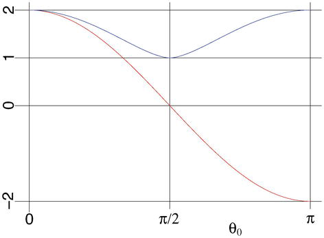
Figure 1.
Weight functions for quantum variance (red) and variance (blue).
Even for large errors, for example a uniform distribution function
In [19], the study of isotropic errors is extended by analyzing the capacity of quantum codes to improve fidelity, and similar results to those presented in [16] are obtained: quantum codes do not improve the fidelity of uncoded quantum states for this type of error.
The results presented in [16, 17, 19] remind us that the quantum computing model is continuous and that the treatment of continuous quantum errors has many subtleties and it is an extraordinarily difficult challenge. Right now we are at a crossroads: extend fault-tolerant quantum computing to error models that include continuous errors or search for a discrete model of quantum computing that allows easier error control. The first road presents formidable difficulties: the fault-tolerant quantum architecture is based exclusively on discrete quantum errors and there is no analogical (continuous) system in the world comparable in complexity to a computer. The second one includes two processes: defining a discrete quantum computing model and finding a quantum system that allows the model to be implemented. It is difficult to know which of the two approaches will lead us to real quantum computing and, for this reason, both should be explored. In this work we study the second one.
A discrete quantum computing model has already been published [20] and, as far as we know, it is the first. In this work Gatti and Lacalle present a discrete quantum computing model based on the following basic requirements:
It describes real states in Quantum Physics.
It preserves the main characteristics of quantum states: superposition, parallelism and entanglement.
It allows to approximate general quantum states.
It contains simple quantum states.
Of all the possible sets of discrete quantum states, there is one that, fulfilling the first three properties, is the most outstanding in terms of simplicity of the states. It is the set of Gaussian coordinate states, which includes all the quantum states whose coordinates in the computation base, except for a normalization factor
To define the model they also need to introduce a set of quantum gates that verify the following properties: it contains quantum gates that transform discrete states into discrete states, and it generates all discrete quantum states. And they includes two elementary quantum gates that verify the above properties,
This quantum gate allows the construction of all Gaussian coordinate states (discrete states) and it is because of this that they call it
This model of discrete quantum computing is related to Number Theory since discrete quantum states
must verify the following diophantine equation:
where
However, we must go one step further with the model of discrete quantum computing, so do not have the same error handling problem again. We need the discrete quantum states to have a basin of attraction associated with them so that any state that falls inside is automatically self-correcting, transforming into the discrete state. This process is used in the manufacture of hardware for classic computers with enormously satisfactory results.
However, Quantum Physics does not allow the application of this process. First of all, self-correction is not a one-to-one transformation and therefore cannot be unitary. And secondly, it cannot be the result of a quantum measurement either because the probability that the result was not the associated discrete state would be greater than zero. Consequently, we need Quantum Physics to go one step further to have the control that discrete quantum computing requires. Is this possible? We believe that this question should have an affirmative answer if the following one does: Is quantum computing possible?
In the following sections we develop further the ideas presented in this introduction.
2. Overview of quantum error control
Today’s quantum error control has two essential components: quantum error correction codes [3, 4, 5, 6, 7, 8] and fault-tolerant quantum computing [9, 10, 11, 12, 13, 14, 15]. There are textbooks on this subject, such as Gaitan’s [22].
2.1 Quantum error correcting codes
Calderbank and Shor [3] and Steane [4] discovered an important class of quantum error correcting codes. The Calderbank-Shor-Steane (CSS) codes are constructed from two classical binary codes. Another approach to the subject originated the quantum stabilizer codes [5, 6, 7, 8]. However, to better understand the role of quantum codes in correcting errors, a general description of them is more useful, without going into the detail of their internal structure.
An quantum error correcting code of dimension
The
That is,
Suppose that a coded state
then the quantum code allows us to retrieve the initial state
An error that does not satisfy Formula (18), that is, it does not belong to
Finally, we want to highlight that discrete errors can be chosen so that, for example, all errors affecting a single qubit are fixed. The best code with this feature that encodes one qubit is the
2.2 Fault-tolerant quantum computing
Fault-tolerant quantum computing was proposed with the aim of proving the quantum threshold theorem or quantum fault-tolerance theorem: a quantum computer with a physical error rate below a certain threshold can, through application of quantum error correction schemes, suppress the logical error rate to arbitrarily low levels. Shor first proved a weak version [9] and the theorem was independently proven by the groups of Aharanov and Ben-Or [15], Knill, Laflamme and Zurek [13] and Kitaev [14].
The essential elements of fault-tolerant quantum computing [9, 13, 15] are as follows: the encoding of each of the qubits with quantum error-correcting codes, the use of fault-tolerant quantum gates, the application of quantum gates on coded qubits (encoded operations) and the concatenation of quantum error-correcting codes.
Another essential element for the proof of the quantum threshold theorem is the quantum error model used. Shor [9] assumes that there is no decoherence error and considers that in a quantum gate an error occurs with probability
Knill, Laflamme and Zurek [13] and Aharanov and Ben-Or [15] consider both decoherence errors and errors in quantum gates and also assume the independence of errors on different qubits. The first [13] analyze quasi-independent and monotonic errors with error strength
In all cases, the parameter
The discretized quantum error model together with the concatenation of error-correcting quantum codes are the key elements in the proof of the quantum threshold theorem. The effect of the conjugation of both is as follows (see for example Figure 6 in [13]):
where we have used the
But this approach cannot be used in all cases, for example for the decoherence error, since in this case the reality is different: the probability of errors occurring in all qubits is
Another key to fault-tolerant quantum computing is to avoid quantum gates that act on two qubits belonging to the same quantum code instance (implementation of fault-tolerant quantum gates for the used quantum code). In this way, the imprecision of the quantum gates only introduces error in at most one qubit of each instance of the quantum code. However, the error in
The use of an instance of an error correcting quantum code of dimension
Finally, it should be noted that the use of quantum codes produces an additional increase in decoherence by increasing the execution time of the algorithms.
Despite the difficulties raised above for the effective control of quantum errors, the discrete quantum error model or stochastic quantum error model allows the proof of the quantum threshold theorem. But unfortunately this model of quantum computing errors does not allow a realistic analysis of continuous quantum computing errors. These break the golden rule of error correction: all small errors must be corrected. The road of fault-tolerant quantum computing goes through including continuous errors in the quantum threshold theorem. This is a huge challenge and for this reason it is interesting to investigate other possible roads.
3. Discrete quantum computing
We are interested in discrete quantum computing because it could lead us to a quantum computing where error control was an easier challenge. In the literature there are some works on discrete quantum computing. They generally intend to simplify or better understand the quantum model: introducing modal concepts and finite fields for the representation of quantum amplitudes [25, 26, 27, 28, 29], using discretization for the design of algorithms [30], relating the structures of computation and the foundations of physics [31, 32, 33, 34, 35, 36, 37, 38] and studying universal sets of discrete quantum gates [39, 40, 41, 42, 43].
As we have already commented in the Introduction, a discrete quantum computing model has already been published [20]. It is a model in which discretization is applied both to quantum states and to quantum gates and that aims to become independent from the standard quantum model (continuous model) and even, if possible, from continuous hardware (Quantum Physics). The presented discrete quantum computing model is based on the following basic requirements:
It describes real states in Quantum Physics.
It preserves the main characteristics of quantum states: superposition, parallelism and entanglement.
It allows to approximate general quantum states.
It contains simple quantum states.
Of all the possible sets of discrete quantum states, there is one that, fulfilling the first three properties, is the most outstanding in terms of simplicity of the states. It is the set of Gaussian coordinate states, which includes all the quantum states whose coordinates in the computation base, except for a normalization factor
To define the model the authors introduce a set of elementary quantum gates that verify the following properties: it contains quantum gates that transform discrete states into discrete states, and it generates all discrete quantum states. This set includes two quantum gates that verify the above properties,
This model of discrete quantum computing is related to Number Theory since discrete quantum states
must verify the following diophantine equation:
where
As we will see in the next subsection, the level of a discrete state is defined as the lowest natural number
where
The superposition principle is also satisfied for non-orthogonal discrete states. For example for the following two discrete states of level
Discrete state
3.1 Discrete quantum states
The quantum gates
They also allow obtaining other quantum gates that are commonly used:
The set of discrete quantum states
The conforming quantum gates
The set of Gaussian coordinate states
Discrete states are classified by levels. We say that a discrete state
Given
Given a number
In discrete quantum computing, the parity and the parity pattern of the coordinates are important. Given a coordinate
From formula (26) it is easy to deduce that the number of coordinates with parity
The proof that the set of discrete states
Therefore, for the state to be reducible, all the coordinates of the state resulting from the application of
The proof starts from a discrete state of level
If all the coordinates are already placed, the state is reducible. Otherwise the first two coordinates will have parity patterns
where
The quantum gate
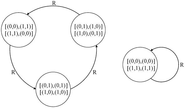
Figure 2.
Rotation of the parity patterns by the quantum gate
3.2 Discrete quantum gates
The introduced discrete quantum computing model satisfies some properties that the authors did not expect to hold. They define discrete quantum gates as the quantum gates that leave the set of discrete states invariant. This means that a quantum gate is discrete if applying it to any discrete state produces another discrete state as a result.
Discrete quantum gates are characterized by a simple property: a quantum gate is discrete if and only if the columns of its matrix, with respect to the computational base, are discrete states with levels of the same parity. This characterization is also fulfilled by substituting the columns of the matrix for the rows, since the matrix is unitary.
The number of discrete gates of one-qubit is finite because the number of discrete states of one-qubit is also finite:
Like discrete states, discrete gates are classified by levels. The level of a discrete gate is defined as the highest of the levels of its columns, considered as discrete states. Obviously if we defined the level of a discrete gate using the rows instead of the columns, the result would be the same.
To proof that a discrete gate can be obtained as a product of gates
Gatti and Lacalle prove it for discrete two-qubit quantum gates and conjecture that the result is true for any number of qubits. To do this, they generalize the properties of the parity patterns already introduced to the discrete gates (see Figure 3). They introduce the following concepts:
Simple match: Given two columns of a discrete gate, we will say that there is a simple match, when there exist elements in both columns, corresponding to the same row, with the real parts or the imaginary parts both odd.
Cross match: Given two columns of a discrete gate, we will say that there is a cross match, when there exist elements in both columns, corresponding to the same row, with the real part of one and the imaginary part of the other both odd.
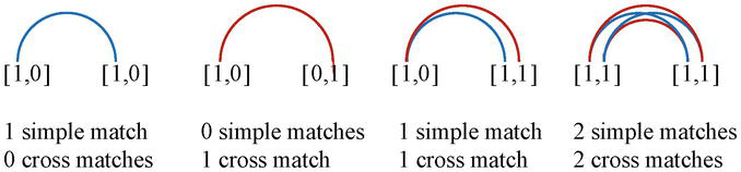
Figure 3.
Odd coordinate component matches.
From this definition and taking into account that the columns of a discrete gate are orthogonal discrete states, we can observe:
The number of odd elements in any column of a discrete gate is even.
Given two columns of a discrete gate, the number of simple matches and the number of cross matches are even.
We remark that every result about the columns of a quantum gate is also valid for the rows, since the matrix is unitary.
As it happened with the quantum states, we need to appeal to the gates
The proof that discrete two-qubit quantum gates can be generated from gates
4. Discrete quantum computing and Lagrange’s four-square theorem
Conjecture 1 can be generalized as follows.
Observe that the conjecture also makes sense for
Before continuing, let us relax the discrete state level definition given in the previous section to any value of
Let us see that, somehow, building a set of orthogonal discrete states is equivalent to completing the set to an orthonormal base. For this reason we will focus in the following problem:
Considering that every discrete
The fact that establishes the connection between discrete quantum computing and Lagrange’s four-square theorem is that the discrete states have to satisfy Eq. (26). Lagrange’s four-square theorem [44] says that every natural number is a sum of four squared integer numbers and, consequently, guarantees that there exist discrete states for any level
Problem 1 is an orthogonal version of Lagrange’s four-square theorem, i.e. the discrete state
Note that given a value of
Problem 1 turns out to be a difficult question in Number Theory and has deep implications. For this reason we begin with the following simplification that most resembles Lagrange’s four-square problem:
Given a natural number
Given a
In this context, the problem we are dealing with (Problem 2) is stated as follows: given a prime number
To prove the result, the authors consider four cases. Three of them are solved with basic linear algebra techniques. However the fourth case is much more difficult, and requires the use of lattices and some Number Theory results.
Case 1: one vector
If the
Case 2: two vectors
If the
Case 3: three vectors
If the
So far, attempts to extend the proof of Problem 2 to arbitrary values of the natural number
If we generalize Problem 2 by applying it to other dimensions, we see that counterexamples can be found for every dimension
In all the problems raised and the conjectures established, the parities of the coordinates are important and, where appropriate, their parity patterns. It is also interesting to note that if we only want orthogonal systems, without specifying the norm or level of the vector with which we want to extend the system, all problems and conjectures are solved affirmatively.
Finally, we want to comment that the authors of the work in which discrete quantum computing is related to Lagrange’s four-square theorem [21], conjecture that Problem 1 has an affirmative answer.
5. Does quantum physics allow discrete quantum computing?
Discrete quantum computing could in principle make error control easier. But in order to take advantage of the fact that quantum states are discrete, Quantum Physics must allow the construction of self-correcting systems. A system with these characteristics associates a basin of attraction with each discrete state so that whenever the
We believe that Quantum Physics can take one step further in the description of physical systems. Quantum Physics still fails to explain fundamental physical concepts, to the point that physicists as relevant as Feynman said “I think I can safely say that nobody understands quantum mechanics” and Quantum Mechanics has a reputation for being especially mysterious.
An example of a surprising result is the the no-cloning theorem [45, 46, 47], which states that it is impossible to create an independent and identical copy of an arbitrary unknown quantum state. This result of Quantum Physics contrasts with the self-reproducing systems of nature and is also derived from the Schrödinger equation, that predicts a unitary evolution of physical systems.
Quantum Physics has so far failed to explain the concepts for which it has acquired the fame of mysterious. We must assume that these mysteries are intrinsic to the nature of physical systems or that there is a road for Quantum Physics to explain them and open new paths for its development. Next we are going to analyze some of the less understandable concepts of Quantum Physics.
The first concept that is difficult to understand is the wave-particle duality. These concepts are inherently incompatible and nevertheless both are necessary to explain many results of Quantum Physics. If we assume that physical systems have a coherent physical description, we must conclude that elementary particles are neither waves nor particles. Therefore they must be something else.
On the other hand, the postulates of Quantum Physics introduce two processes to describe the evolution of physical systems: the Schrödinger equation and quantum measurements. The first predicts a unitary evolution of physical systems while the second seems to violate the prediction of the first. Many researchers assume that the result of the measurement of a quantum system is a random process whose probabilities depend on the measured system and not on the device that performs the measurement, and that the result is random, that is, there are no hidden variables that determine the result deterministically. In this interpretation the measurement process violates the Schrödinger equation. Other interpretations regard quantum states as statistical information about quantum systems, thus asserting that abrupt and discontinuous changes of quantum states are not problematic, simply reflecting updates of the available information. These reinforce the mysterious character of Quantum Physics and change its objective of describing physical systems for that of only obtaining information.
Finally, we want to comment on the interpretations made of the wave function obtained by solving the Schrodinger equation. It is common to hear that the wave function, for example of an electron, does not indicate that the particle is at all points where the wave function is not zero and that it is not an indicator of our ignorance of the position of the particle. On the one hand we give all the credit to the Schrödinger equation and on the other we take it away from the wave function.
As we see the controversy continues to haunt Quantum Physics. From our point of view, Quantum Physics has found a prediction system for the results of the measurements of physical systems, but it does not describe them. This prevents Quantum Physics from advancing in the deductive knowledge of physical systems, leaving only the advance based on experimentation. Does Quantum Physics really describe everything we can know about physical systems? We do not believe it.
What can be done to get out of this loop? We believe that we should focus on the initial problem: the wave-particle duality. As we have indicated before, this dilemma indicates that elementary particles are neither waves nor particles. Therefore the first objective is to determine its nature. To do this, we must look for questions that can be answered through the design of experiments and that shed light on the nature of elementary particles. In our opinion the first important question is the following: In how many points of space can an elementary particle be simultaneously?
Physics, in addition to the problems of Quantum Physics already mentioned, also has serious problems to combine two of its most notable theories: General Relativity and Quantum Physics. Undoubtedly, any theory that goes in the direction of discretizing space must also consider the discretization of time. In our study we only intend to contribute ideas so that Quantum Physics can overcome the controversies that it is not able to explain. We do not start from the hypothesis that Quantum Physics must be a discretized theory, but we believe that it must be a theory that allows self-correction and that this property must allow the implementation of a discrete quantum computation.
In Quantum Physics, different types of discretization have been proposed, in addition to the one presented in this article. Thus, in [48] a discretization of the quantum state space is proposed in order to explain Born’s rule for probabilities. The proposal, despite being very similar to the one we have presented in this article, has very different objectives. In [48] it is used to try to explain two of the most important interpretations of Quantum Physics: Many Worlds and Copenhagen interpretation. In our case the objective is to define a discrete quantum computing model allowing effective control of quantum errors. And this objective leads us to pose an important question, aimed at explaining the wave-particle duality: In how many points of space can an elementary particle be simultaneously?
5.1 Hypothesis on the nature of elementary particles
Elementary particles cannot be in only one position in space because they cannot explain their behavior as waves. Then, in how many positions can they be simultaneously? The answer can be a finite number greater than one, a countable infinite number, or even an uncountable infinite number. Due to the principle of simplicity, we are inclined to take as a working hypothesis that the answer is a finite number greater than one.
And what does it mean for a particle to be simultaneously at various points in space? In our hypothesis the particle orbit between all its possible positions but being in only one at each time. Therefore simultaneity must be taken in a non-strict sense. That a particle orbits in different points means that it disappears from one point and appears in another and so on. The particle does not travel from one point to another through ordinary space and, in this sense, it may violate the special relativistic principle of speed limitation. Colloquially speaking the particle travels through a “wormhole”, without deforming space through large concentrations of mass.
And, why do we choose this elementary particle model as a hypothesis? Because as we have said, the particle must be able to be in more than one point simultaneously and there are already experimental results of quantum nonlocality [49, 50, 51, 52, 53]. As far as we know, quantum nonlocality does not allow for faster-than-light communication and it is generally assumed that is compatible with special relativity and its universal speed limit of objects. We believe that quantum nonlocality in some sense violates the aforementioned principle of special relativity. We do not believe that the physical characteristics of the systems should be subordinated to the ability to transmit information.
From our point of view, the multi-position structure of the particles generates nonlocality in the usual space and breaks its Euclidean behavior. In this way physical systems can interact non-locally in space through their multi-position structure.
Another question that arises naturally from our working hypothesis is how scattered can the points that define an elementary particle be in space? Non-point particles can naturally explain their intrinsic angular momentum and this, in turn, give us information about the structure of the particles. For example, a particle that could be in three points in space would have an angular momentum proportional to the area of the triangle determined by its positions. This would indicate that the dispersion of the particles would occur on typical scales of Quantum Physics.
The multi-position particle hypothesis would again bring up some problems that originated Quantum Theories, such as, for example, the stability of atoms. This problem would be solved by the spatial scattering of the electrons around the nucleus. In this case the far electromagnetic field generated by the electrons would decrease faster than the inverse of the square of the distance and this would prevent the electrons from losing their energy in the form of electromagnetic radiation.
Our hypothesis would force us to readapt Quantum Theory. Therefore, we should plan experiments that allow us to contrast it. Is this possible?
5.2 How to test the hypothesis experimentally?
We would like to propose a couple of experiments that could theoretically provide information on our hypothesis about the structure of elementary particles. The first is a variation of the flagship experiment in which the wave-particle duality of elementary particles is tested: the double-slit experiment. The second uses a known quantum effect: the quantum tunneling.
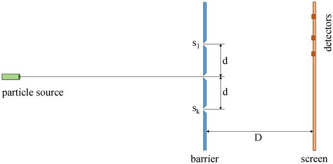
Figure 4.
The objective of this experiment is to determine if the particles, according to our hypothesis, can be simultaneously in exactly
We start the experiment by choosing
It would be necessary to estimate if the measurements can be precise enough to distinguish the two patterns and, in the first, if the probability of the
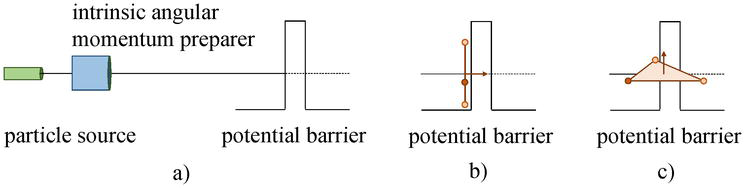
Figure 5.
Quantum tunneling experiment.
The objective of this experiment is to determine if the state of the particles influences the probability of quantum tunneling. If this influence is confirmed, it would mean that the orientation of the intrinsic angular momentum of the particles determines in some way the internal structure of the particle against the potential barrier. This could be explained quite understandably with the hypothesis that the particles are in exactly
We believe that it is not difficult to design more experiments that can shed light on our hypothesis of elementary particles. At this moment we are studying the dynamics of these multi-position particles.
6. Conclusions
In this article we introduce the discrete quantum computing as an alternative road to real quantum computing. The discrete quantum computing model is of great interest in itself both because, while maintaining all the important properties of quantum computing, it is an especially simplicity model and because error control is theoretically easier in this model. The introduced discrete quantum computing model satisfies some surprising properties that the authors believed would not hold and has deep connections to Number Theory.
The reason we set out on this alternative road to quantum computing is because error control in quantum computing is an extremely difficult challenge. The fact that the quantum computing model is continuous means that the golden rule of error control cannot be used: small errors are exactly corrected. A quantum computer is a very complex system from the point of view of error control. It allows reaching any quantum state (solution to the instance of a problem) by any path (algorithm). Doing this while keeping the error (entropy?) controlled is certainly an impressive challenge. As a consequence of the difficulty of controlling errors in continuous systems, there is no analog (continuous) device remotely comparable in operational complexity to a computer.
However, Quantum Physics does not allow the implementation of a discrete quantum computing model that allows self-correction of errors. To overcome this difficulty we ask Quantum Physics to go one step further in describing physical systems, beyond the prediction of measurement results. For this we propose a hypothesis about the nature of elementary particles that tries to overcome the never-understandable principle of wave-particle duality.
Summarizing, we propose an alternative road to quantum computing that passes through the discretization of this computing model and overcoming the interpretation gaps of Quantum Physics relative to the physical systems.
References
- 1.
Marella S T, Parisa H S K. Introduction to Quantum Computing. In: IntechOpen. DOI: 10.5772/intechopen.94103. Available from: https://www.intechopen.com/online-first/introduction-to-quantum-computing - 2.
Nielsen M A, Chuang I L. Quantum Computation and Quantum Information. Cambridge University Press; 2010. 664 p. DOI: 10.1017/CBO9780511976667 - 3.
Calderbank A R, Shor P W. Good quantum error-correcting codes exist. Phys. Rev. A. 1996;54:1098–1105 - 4.
Steane A M. Multiple particle inference and quantum error correction. Proc. Roy. Soc. A. 1996;452:2551 - 5.
Gottesman D. Class of quantum error correcting codes saturating the quantum Hamming boud. Phys. Rev. A 1996;54:1862 - 6.
Calderbank A R, Rains E M, Shor P W, Sloane N J A. quantum Error Correction and Orthogonal Geometry. Phys. Rev. Lett. 1997;78:405 - 7.
Gottesman D. Stabilizer Codes and Quantum Error Correction [thesis]. California Institute of Technology; 1997 - 8.
Calderbank A R, Rains E M, Shor P W, Sloane N J A. quantum error correction via codes over GF(4). IEEE Trans. Inf. Theory. 1998;44(4):1369–1387 - 9.
Shor P W. Fault-tolerant quantum computation. In: Proceedings of 37th Conference on Foundations of Computer Science; 14-16 October 1996; Burlington, VT, USA. IEEE Comput. Soc. Press; 1996. p. 56–65. arXiv:quant-ph/9605011. DOI: 10.1109/SFCS.1996.548464 - 10.
Steane A M. Active stabilization, quantum computation and quantum state synthesis. Phys. Rev. Lett. 1997;78:2252 - 11.
Preskill J. Reliable quantum computers. Proc. Roy. Soc. Lond. A. 1998;454:385–410 - 12.
Gottesman D. Theory of fault-tolerant quantum computation. Phys. Rev. A. 1998;57:127–137 - 13.
Knill E, Laflamme R, Zurek W H. Resilient Quantum Computation. Science. 1998;279(5349):342–345. arXiv:quant-ph/9702058v1. DOI: 10.1126/science.279.5349.342 - 14.
Kitaev A Yu. Fault-tolerant quantum computation by anyons. Annals of Physics. 2003;303(1):2–30. arXiv:quant-ph/9707021. DOI: 10.1016/S0003-4916(02)00018-0 - 15.
Aharonov D, Ben-Or M. Fault-Tolerant Quantum Computation with Constant Error Rate. SIAM Journal on Computing. 2008;38(4):1207–1282. arXiv:quant-ph/9906129. DOI: 10.1137/S0097539799359385 - 16.
Lacalle, J., Pozo-Coronado, L.M., Fonseca de Oliveira, A.L., Quantum codes do not fix isotropic errors. Quantum Inf Process 20, 37 (2021). https://doi.org/10.1007/s11128-020-02980-3 - 17.
Lacalle J, Pozo Coronado L M, Fonseca de Oliveira A L, Martín-Cuevas R. Quantum codes do not fix qubit independent errors. Will appear in American Journal of Information Science and Technology. 2021. arXiv:2101.03971 [quant-ph] - 18.
Lacalle J, Pozo Coronado L M. Variance of the sum of independent quantum computing errors. Quantum Information & Computation. 2019;19(15-16):1294–1312. DOI: 10.26421/QIC19.15-16 - 19.
Lacalle J, Pozo Coronado L M, Fonseca de Oliveira A L, Martín-Cuevas R. Quantum codes do not increase fidelity against isotropic errors. Personal communication 2021. It will appear in arXiv [quant-ph] - 20.
Gatti L N, Lacalle J. A model of discrete quantum computation. Quantum Inf Process. 2018;17(192). DOI: 10.1007/s11128-018-1956-0 - 21.
Lacalle J, Gatti L N. Discrete quantum computation and Lagrange’s four-square theorem. Quantum Inf Process. 2020;19(34). DOI: 10.1007/s11128-019-2528-7 - 22.
Gaitan F. Quantum error correction and fault tolerant quantum computing, CRC Press; 2008. 292 p - 23.
Bennet C H, DiVincenzo D P, Smolin J A, Wootters W K. Mixed state entanglement and quantum error correction. Los Alamos Physics Preprint Archive. 1999. arXiv:9909058 [quant-ph] - 24.
Laflamme R, Miquel C, Paz J-P, Zurek W H. Perfect quantum error correction codes. Phys. Rev. Lett. 1996;77:198. arXiv:9602019 [quant-ph] - 25.
Benjamin S, Westmoreland M D. Modal quantum theory. Found. Phys. 2012;42(7):918-–925 - 26.
Ellerman D. Quantum mechanics over sets. arXiv:1310.8221v1 [quant-ph] - 27.
Hanson A J, Ortiz G, Sabry A, Tai Y-T. Geometry of discrete quantum computing. J. Phys. A Math. Theor. 2013;46(18):185301 - 28.
Hanson A J, Ortiz G, Sabry A, Tai Y-T. Discrete quantum theories. J. Phys. A Math. Theor. 2014;47(11):115305 - 29.
Gatti L N, García-López J. Geometría de estados discretos en computación cuántica. In: 10th Andalusian Meeting on Discrete Mathematics; July 10-11, 2017; La Línea de la Concepción, Cádiz, Spain - 30.
Chandrashekar C M, Srikanth R, Laflamme R. Optimizing the discrete time quantum walk using a su(2) coin. Phys. Rev. A. 2008;77:032326 - 31.
Lloyd S, Dreyer O. The universal path integral. Quant. Inf. Process. 2016;15(2):959–967 - 32.
Long G-L. General quantum interference principle and duality computer. Commun. Theor. Phys. 2006;45(5):825 - 33.
Long G-L, Liu Y. Duality computing in quantum computers. Commun. Theor. Phys. 2008;50(6):1303 - 34.
Long G-L, Liu Y, Wang C. Allowable generalized quantum gates. Commun. Theor. Phys. 2009;51(1):65 - 35.
Gudder S. Mathematical theory of duality quantum computers. Quant. Inf. Process. 2007;6(1):37–48 - 36.
Long G-L. Mathematical theory of the duality computer in the density matrix formalism. Quant. Inf. Process. 2007;6(1):49–54 - 37.
Wei S-J, Long G-L. Duality quantum computer and the efficient quantum simulations. Quant. Inf. Process. 2016;15(3):1189–1212 - 38.
Lomonaco S J. How to build a device that cannot be built. Quant. Inf. Process. 2016;15(3):1043–1056 - 39.
Kitaev A Y, Shen A, Vyalyi M N. Classical and Quantum Computation. American Mathematical Society. Providence; 2002;47 - 40.
Oscar B P, Mor T, Pulver M, Roychowdhury V, Vatan F. On universal and fault-tolerant quantum computing: a novel basis and a new constructive proof of universality for shor’s basis. In: 40th Annual Symposium on Foundations of Computer Science; October, 17-19,1999; New York City, NY, USA - 41.
Shi Y. Both toffoli and controlled-not need little help to do universal quantum computing. Quant. Inf. Comput. 2003;3(1):84–92 - 42.
Aharonov D. A simple proof that Toffoli and Hadamard are quantum universal. arXiv:0301040 ][quant-ph] - 43.
Kliuchnikov V, Maslov D, Mosca M. Fast and efficient exact synthesis of single qubit unitaries generated by Clifford and T gates. Quant. Inf. Comput. 2013;13(7–8):607–630 - 44.
Lagrange J L. Démonstration d’un théorème d’arithmétique, Oeuvres complétes 3 ; 1869. 189–201 - 45.
Park J. The concept of transition in quantum mechanics. Foundations of Physics. 1970;1(1):23–33. DOI: 10.1007/BF00708652 - 46.
Wootters W, Zurek W. A Single Quantum Cannot be Cloned. Nature. 1982;299(5886):802–803. DOI: 10.1038/299802a0 - 47.
Dieks D. Communication by EPR devices. Physics Letters A. 1982;92(6):271–272. DOI: 10.1016/0375-9601(82)90084-6 - 48.
Buniy R V, Hsua S D H, Zee, A. Discreteness and the origin of probability in quantum mechanics. Physics Letters B. 2006;640: 219–223. DOI: 10.1016/j.physletb.2006.07.050 - 49.
Aspect A, Dalibard J, Roger G. Experimental Test of Bell’s Inequalities Using Time- Varying Analyzers. Physical Review Letters. 1982;49(25):1804–1807. DOI: 10.1103/PhysRevLett.49.1804 - 50.
Rowe M, Kielpinski D, Meyer V et al. Experimental violation of a Bell’s Inequality with efficient detection. Nature. 2001;409(6822):791–794. DOI: 10.1038/35057215 - 51.
Hensen B, Bernien H, Dréau A et al. Loophole-free Bell inequality violation using electron spins separated by 1.3 kilometres. Nature. 2015;526(7575):682–686. DOI: 10.1038/nature15759 - 52.
Giustina M, Versteegh M A M et al. Significant-Loophole-Free Test of Bell’s Theorem with Entangled Photons. Physical Review Letters. 2015;115(25):250401. DOI: 10.1103/PhysRevLett.115.250401 - 53.
Shalm L K, Meyer-Scott E et al. (December 2015). Strong Loophole-Free Test of Local Realism. Physical Review Letters. 2015;115(25):250402. DOI: 10.1103/PhysRevLett.115.250402