Analysis of Solution Diversity in Topic Models for Smart City Applications

1. Introduction

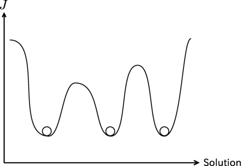
Probabilistic latent semantic analysis (PLSA: probabilistic latent semantic analysis) [1] and latent Dirichlet analysis (LDA: latent Dirichlet allocation) [2] are known as topic models to analyze count data such as documents (text data). In a smart city, it is important to collect and analyze citizens’ voices to discover their concerns and issues. Topic modeling is effective for the above analysis because it can extract topics from a collection of documents. However, when estimating parameters (solutions) in topic models, various solutions are reached due to differences in algorithms and initial values. There could exist a lot of local optimal solutions that are distinct but are equally optimized in the objective function (Figure 1). Since each of these solutions presents an interpretation of data, they are meaningful and worth using. In order to select a solution suitable for the purpose from among the various solutions, it is necessary to know what kind of solutions exist. This chapter introduces methods for analyzing diverse solutions and obtaining an overall picture of the solutions.

The solution, which is the set of parameters estimated in topic models, has a topic distribution θ and a word distribution ϕ. A topic distribution θ is tied to each document, and it represents the mixture ratio of topics in the document. The word distribution ϕ represents the probability of occurrence of each word in a topic. The methods presented here analyze diverse solutions using topic and word distributions, respectively.

The method [3, 4] using topic distribution θ defines the normalized mutual information (NMI) [5] that can be calculated for two solutions as the similarity between them, and assign coordinate values to them by multidimensional scaling (MDS) [6]. The coordinate values can be used to visualize the distribution of solutions in low-dimensional space.

Word distribution ϕ directly represents topic characteristics and is easy for humans to understand, making their analysis valuable. Specifically, clustering and network representation of similar relations are used to obtain groups of word distributions that are similar to each other. Each solution is then typified based on the frequency distribution of the groups. As a result, several typical solutions and word distributions that could be taken were successfully represented in a human-understandable form [7].

The related studies are shown below. As for analyzing multiple solutions, there are studies on clustering. In these studies, the Rand index or NMI is used to define the distance or similarity between solutions. Then, a non-redundant alternative solution for a given solution is found [8], several non-redundant are searched [9], and solutions are visualized by dendrogram [10]. This chapter focuses on topic model which includes hard clustering as a special case. The article [11] is a study of visualizing the solution of a topic model, but for a single solution. Few studies analyze and visualize multiple solutions in topic models.

The experiments deal mainly with text data of news articles and show the distribution of the solutions and the typical topics in the topic model. We expect that the proposed methods will contribute to the discovery of problems in smart cities.

2. Topic models and estimation of its solution

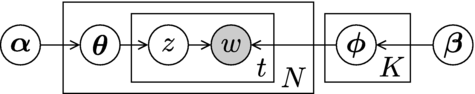
Topic models could be described by a generative probability model as shown in Figure 2. Shaded circles represent observed variables and white circles represent unobserved variables. The square plates represent repetitions, and the number in the lower right corner indicates the number of repetitions. Items inside the plate are conditionally independent given the variable outside the plate. In fact, the observed variables are “words” and the observed data, which is the accumulation of these words, is a document.

Assume that there are topics kk=1…K, document ii=1…N, and M types of words in the total of documents. Also, assume that each topic k has a word distribution ϕk=ϕ1k…ϕmk…ϕMk and the document has a topic distribution θi=θ1i…θki…θKi. For each document i, the following is repeated ti times. A topic z is assigned based on the topic distribution θi, and a specific word w is generated based on the word distribution ϕz. All words generated for document i are aggregated by type and made into an observed value vector xi=w1i,…,wMi, where wmi denotes the frequency of m-th word. Hence, l1-norm of i-th observed value vector ∑m∣xmi∣ equals ti. All observed value vectors are denoted by X=x1…xN, which is the vector representation of all documents. α and β are hyperparameters for the prior probability distributions of the topic distribution θ and the word distribution ϕ respectively, and a uniform Dirichlet distribution is assumed here.

Given the probability Pmi that word m is generated in document i, PkiPmk=θkiϕmk if the k-th topic is assigned, so Pmi=∑k=1Kθkiϕmk considering all topics. The number of words m in document i equals xmi, and all word generations are independent. Therefore, the simultaneous probability for all document generations can be represented by a multinomial distribution

where Ai is the number of combination for document i. Taking the logarithm of Eq. (1) yields

The first term is a constant for the observed value vectors X, and the second term is the objective function to be maximized, when inferring parameters. A set of parameters θϕ of this function is a solution to be inferred. In the experiment, we use the equivalent perplexity:

There are various algorithms for estimating the model parameters, including collapsed Gibbs sampling (CGS) [12], variational Bayesian estimation (VB) [2], collapsed variational Bayesian estimation (CVB) [13], maximum likelihood estimation (ML) [1], maximum a posteriori probability (MAP) estimation [14]. From these, we use MAP estimation, CGS as a sampling approximation method, and CVB0 [15], which uses zero-order approximation of CVB, as a variational approximation method to estimate diverse solutions.

The update formulas used in the iterations in MAP estimation of θ,ϕ are

where ηmk is the number of occurrence about the word of type m at topic k and ηki is the number of assignment of topic k to data i. These can be calculated by

The updates at each iteration in CGS estimation can be written as

using the sampled topic set. When sampling for the j-th word wij in data i, the probability that the topic is k when the type of this word is m follows

where \ij denotes that the information about the word wij under focus is excluded, and Z\ij denotes the topic set excluding the topic zij of the word wij.

In CVB0 estimation, for the j-th word wij in data i, the burden rate that the topic is k when the type of this word is m follows

The expectations of ηmk and ηki are respectively estimated by Eηmk=∑i,j∣wij=mρijk and Eηki=∑jρijk. Estimation of ϕmk and θki are obtained by

Estimation in CVB0 proceeds by alternating between estimating ϕmk and θki and updating the burden rate ρijk in Eq. (8) [15].

Initial value setting using information-theoretic clustering is applicable in MAP estimation. It was shown that weighted information-theoretic clustering is a special case of topic models (see Appendix A), and it was confirmed that using the clustering results for initial value setting yields a better solution than using random initial value setting [16]. Specifically, the method is to smooth the word distribution obtained from clustering by adding a small value and use it as the initial word distribution ϕ.

3. An analysis method using topic distribution

This section presents the method [3, 4] to assign coordinate values to solutions using the topic distribution θ. This allows visualization of solutions.

The Normalized Mutual Information (NMI) is known as external criterion for evaluation of clustering [5], but can be applied to solutions in topic models as follows.

There are two solution, A and B for the same set of documents. A has J topics Ajj=1…J and B has K topics Bkk=1…K. The topic distribution of document ii=1…N for A and B are denoted by θji and θki, respectively. Then, the degree of simultaneous sampling of topic Aj and topic Bk can be expressed as tiθjiθki, where ti is the number of words included in document i. Integrating the degree of simultaneous sampling across the entire document set yields

which represents the overlap between Aj and Bk. Hence, we obtain a confusion matrix (Table 1) with DgAjBk as an element. The total degree, say T, equals the number of words in the total of documents ∑i=1Nti, since ∑jθji=∑kθki=1∀i.

Table 1 is a frequency distribution. Dividing this by the total frequency yields a two-dimensional probability distribution. The simultaneous probability is given by

Using the simultaneous probabilities PAjBk, the NMI between two solutions (discrete random variables) A and B is defined as [5]

where IAB is the mutual information and H is the entropy. Specifically

Since a symmetrical relationship NMIAB=NMIBA is satisfied from above, NMI can be thought of as a similarity related to information and also as an inner product between solutions.

Let θll=1…L be a set of solutions about topic models. Forming the inner product matrix BL×L whose elements are the inner products calculated as NMI between them, then the matrix B enables us to assign coordinate values to the solutions by multidimensional scaling (MDS) [6].

Let yl, Y=y1…yL be the coordinate value (vector) of l-th solution in Euclidean space, and the matrix expression of them, respectively. B as the inner product matrix can be expressed by

Since B is symmetric and positive semidefinite from the definition of NMI, there exists an orthogonal matrix Φ such that

where Λ is a diagonal matrix whose elements are eigenvalues of B. Hence,

and we obtain

The vectors Y can be used to visualize the solutions in low-dimensional space. The eigenvalue decomposition in (Eq. (17)) is for the origin viewpoint and not the center of gravity, so when applying principal component analysis (PCA), it should again be applied to the vectors Y.

4. An analysis method using word distribution

This section introduces the method [7] for representing typical solutions and the topics contained therein, as well as possible topics that can be extracted, by means of the word distribution ϕ that are easy for human to understand. Considering all word distributions in diverse solutions, the number of combinations of word distributions is enormous. It is inefficient to treat “quite similar” and “different but similar” relationship equally in order to get a complete picture of word distributions. Therefore, we represent the former relationships by grouping them together under the same representative word distribution and the latter relationships by analysis based on similarity relations among representative word distributions. These are described in detail below.

Information-theoretic clustering [16, 17] based on similarity of probability distributions is used to estimate representative word distributions from word distributions ϕ1…ϕi…ϕN included in solutions. The objective function to be minimized in this clustering is expressed as

where DKL denotes Kullback-Leibler divergence, Cf is the estimated cluster of word distributions that are quite similar to each other, and Qf is the estimated representative word distribution, which is literally representative of the word distributions that could be extracted in topic modeling. The number of clusters Kf should be large enough so that they consist of word distributions that are quite similar to each other.

Representative word distributions with similar relationships are then connected to form similarity network of representative word distributions. Whether representative word distributions ϕi and ϕj are similar or not is determined by Jensen Shannon (JS) divergence given as

In this network, there are groups of representative word distributions that are similar to each other in areas of high edge density. These groups are extracted by the clustering algorithm based on maximizing modularity [18].

Since word distributions belong to one of the groups via the representative word distribution, solutions can be typified by the frequency distribution of the group to which the included word distribution belongs. As a result, several typical solutions can be found by the analysis using word distributions.

5. Experiments

We used three text data sets: NYtimes [19], 20News [20], Nips [19]. Stop-words included in 20News and documents with fewer than 40 words were removed. The characteristics of data sets actually used are shown in Table 2.

Each data set was separated into a training set for 90% of its documents and a test set for 10%. The test set were used to evaluate parameter estimation. The parameters θ,ϕ, which are the solutions estimated for the training set, were analyzed. The methods used are (1) MAP estimation (MapRnd), (2) MAP estimation using information-theoretic clustering results for initial value setting (MapCL), (3) collapsed Gibbs sampling (CGS), and (4) collapsed variational Bayesian estimation (CVB0). Of these, random initial values were given to the parameters in all cases except (2), where a small value was added to each element of the word distribution of the cluster obtained by weighted information-theoretic clustering to make the initial word distributions ϕ and a uniform distribution was set as the initial topic distribution θ [16].

The number of topics was set to K=10, and the hyperparameters were set to α=1.01 and β=1.1 for MAP estimation and α=0.01 and β=0.1 for the other methods, adjusting for differences in the update equations [15]. For each method, parameter estimation was performed for 200 different random number series.

5.1 Experimental results

We evaluated a total of 800 solutions θϕ, estimated and acquired through the four methods, by perplexity calculated using the test set (Table 3). With the acquired ϕ as known, the topic distribution θtest was estimated using half of the words in each document in the test set, and the perplexity was calculated from the word and topic distributions ϕ,θtest using the other half of the words. Since the objective is to evaluate the goodness of solution, the estimation of the topic distribution in the test set is the same for all methods, and MAP estimation was used in this case. Table 3 shows that MapCL, which uses clustering results as initial values, is superior to MapRnd, and that Cvb0 performs better than the other methods except MapCL. The fact that Cvb0 shows better results is consistent with the results in [15].

Name	MapRnd	MapCL	Cgs	Cvb0
NYtimes	5983.8	5959.3	5991.7	5973.7
20News	5693.3	5662.4	5772.7	5688.9
Nips	1993.3	1989.3	2006.4	1982.3

Table 3.

Perplexities archived in the four methods.

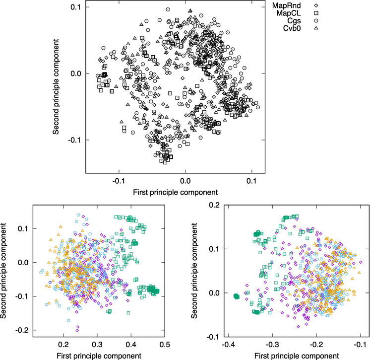
We assigned coordinate values to the solutions by the analysis using topic distributions and applied principal component analysis PCA to visualize them in Figure 3.

In Figure 3, we see that MapCL is biased toward the range of large (20News) and small (Nips) values of the first principal component. This indicates that the solutions are method-dependent. These diagrams are useful to get an overall picture of the distribution of solutions, and by choosing solutions far from each other (e.g., top left, top right, center, bottom left, bottom right), a non-redundant solution set is obtained. However, how they differ is difficult for humans to understand. Therefore, it is important to analyze using word distributions that are easy for humans to understand.

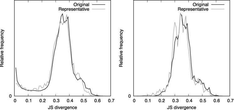
For the analysis using word distributions, 100 representative word distributions were first obtained by information-theoretic clustering (see Eq. (19)) from a total of 8000 word distributions, 10 in each solution. The frequency distributions of JS divergence between word distributions and JS divergence between representative word distributions are shown in Figure 4 (left). Since the two frequency distributions are well matched, and the representative word distributions preserve the relationships among the word distributions, Kf=100 would be sufficient for the number of clusters.

Figure 4 (right) shows the frequency distribution of the JS divergence between word distributions inside each solution and between representative word distributions corresponding to the word distributions. The word distributions in the solution of topic models are estimated to be different from each other in the sense of optimizing the objective function (Eq. (2)). Therefore, the JS divergence between word distributions inside the solution has a larger value. Considering this figure, we determined that word distributions are similar to each other if the JS divergence between them is equal to 0.1 or less.

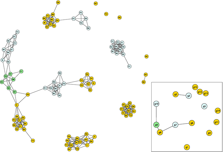
We then connected representative word distributions with similar relationships for the NYtimes data set and represented them as a similarity network of representative word distributions in Figure 5. From this network, the clustering algorithm based on maximizing modularity [18] was used to extract groups (g1 to g15) with representative word distributions that were in regions of high edge density. There were 10 large groups with four or more vertices, the same as the number of topics K. In Figure 5, the vertices are colored to distinguish the groups and only the network information representing the adjacencies is meaningful, not the positions (coordinate values) of the vertices.

Table 4 shows the high-frequency words in the representative word distributions for each large group (g1 to g10) in NYtimes. For the adjacent and ambiguous groups (g6 to g10) in Figure 5, two representative word distributions were chosen to represent the variation within the group, and the characteristic words representing the differences are shown in bold. The words “school student” appear in g6, g7, and g8, suggesting that there are a variety of topics related to these words. We see that the word “drug” is listed with “doctor” in g6, but with “case” in g7.

gn	fn	High-frequency words
g1	f41	team game season player play games point run coach win won right hit left
g2	f40	company percent million companies market stock business billion money
g3	f22	com web computer site information www mail online .internet internet
g4	f55	.bush president campaign .george_bush .al_gore election political vote
g5	f36	official government .united_states .u_s military war attack palestinian leader
g6	f2	drug patient doctor cell research problem scientist percent health study
	f70	school student drug patient percent program doctor women study problem
g7	f16	school case student drug law court official patient children lawyer found
	f51	school student family children case home told police death law lawyer official
g8	f76	school student children family women home friend father mother parent
	f61	show book film movie look music friend women play family character love
g9	f20	home family room building friend night house children town .new_york
	f37	car building water room home air hour area miles town house feet place
g10	f6	water food room cup minutes small building hour restaurant add large home
	f72	food cup minutes add water oil restaurant wine tablespoon fat sugar chicken

Table 4.

High-frequency words in the representative word distribution for each group in NYtimes.

The representative word distributions within these groups are somewhat different, and it is not easy to select the appropriate one. Therefore, the proposed method of representing relationships in a human-understandable form may be useful for users. If we were to name the groups according to the high-frequency words, they would be, in order, sports (g1), markets (g2), IT (g3), presidential election (g4), international conflicts (g5), health care (g6), school (g7), entertainment (g8), housing (g9), and food (g10).

We typified solutions by the frequency distribution of the group to which the word distribution in the solution belongs. We call the types of frequency distributions patterns, and the top five most frequently occurring patterns are listed in Table 5. As the tables show, these patterns consist of combinations of the large groups (g1 to g10). For patterns 1 and 2, we selected solutions that are typical in the sense that we often find combinations of representative word distributions associated with the word distributions in the solution, and listed in Table 6 the high-frequency words in the word distributions belonging to these solutions. In the tables, the names of the groups to which the word distributions belong are indicated.

	g1	g2	g3	g4	g5	g6	g7	g8	g9	g10	Number
Pattern 1	2	1	0	1	1	1	1	1	1	1	125
Pattern 2	1	1	1	1	1	1	1	1	1	1	81
Pattern 3	2	1	1	1	1	1	1	1	0	1	67
Pattern 4	2	1	1	1	1	0	1	1	1	1	66
Pattern 5	1	1	0	1	1	1	1	2	1	1	46

Table 5.

High-frequently occurring patterns. “Number” indicates the number of solutions belonging to the pattern.

Group name	High-frequency words
Sports	season team game run games hit player inning play baseball right
Sports	team game season player play point games coach win won yard
Markets	company percent million companies market business stock billion
Presidential election	.bush president campaign .george_bush .al_gore election political
International conflicts	official government .united_states attack .u_s military war leader
Health care	drug patient doctor percent problem cell research study health
School	school student case law court lawyer children police official family
Entertainment	show book film movie music look play women friend character
Housing	car building home room water hour house area air town miles
Food	cup food minutes add oil tablespoon wine sugar pepper water

Group name	High-frequency words
Sports	team game season player play games point run coach win football
Markets	percent company million companies market stock business billion
IT	com web computer information site www mail online .internet
Presidential election	.bush campaign president .george_bush .al_gore election political
International conflicts	official government .united_states attack .u_s military war leader
Health care	drug patient doctor health research study scientist cell problem
School	school student law case court lawyer official children police family
Entertainment	show film book movie look women play music friend character
Housing	car building home room water hour house town miles area air
Food	cup food minutes add oil wine tablespoon sugar pepper

Table 6.

High-frequency words in typical solutions for pattern 1 (top) and pattern 2 (bottom).

As Table 6 (top) shows, the pattern 1 has no topics on IT and instead has two topics on sports. The pattern 3 has no topics related to housing in g9 (see Table 5). If we were to have the right set of topics for a smart city, we should choose a solution from the pattern 2 (see Table 6 (bottom)), which includes the all groups, rather than focusing on sports.

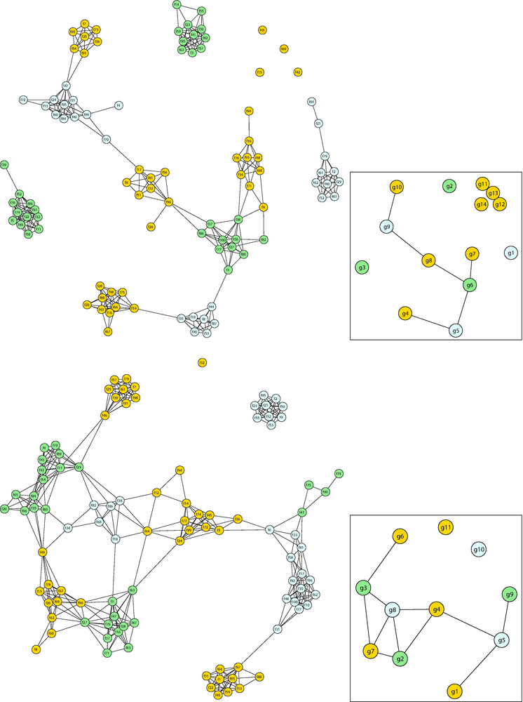
Figure 6 shows similarity networks of representative word distributions for the 20News and Nips data sets. As these figures show, for both data sets, the number of large groups was 10, the same as the number of topics.

The 20News and Nips solutions were typified based on the frequency distribution of the groups, and the top five most frequently occurring patterns are shown in Table 7. As the tables show, these patterns also consist of combinations of the large groups (g1 to g10). Since large groups play a role in many solutions, a solution with one word distribution for all large groups would be the solution of interest. However, such a solution is not necessarily the most common solution, nor is it necessarily the optimal solution. For reference, Table 8 shows examples of such solutions. The 20News example belongs to the most common pattern (pattern 1) and could be a candidate for a good solution. In the 20News data set, documents are labeled with the newsgroup to which they belong [20]. Using the label information, we can find the high-frequency words of the documents belonging to each newsgroup (see Table 9). Note that topic modeling does not use label information. Comparing the topics in Table 8 (top) with those in Table 9, many of them are associated. For example, g1 is associated with n11, g3 with n8–9, g4 with n15, g5 with n14, and g9 with n2. This association with the actual newsgroups would supports that the solution in Table 8 (top) is appropriate. The Nips example belongs to the fourth most common pattern, and a solution to the other patterns would be appropriate.

	g1	g2	g3	g4	g5	g6	g7	g8	g9	g10	Number
Pattern 1	1	1	1	1	1	1	1	1	1	1	215
Pattern 2	2	1	1	1	1	1	1	0	1	1	44
Pattern 3	1	2	1	1	1	1	1	0	1	1	39
Pattern 4	1	2	1	1	0	1	1	1	1	1	29
Pattern 5	1	1	1	1	1	1	2	0	1	1	27

	g1	g2	g3	g4	g5	g6	g7	g8	g9	g10	Number
Pattern 1	1	1	2	1	2	1	1	0	0	1	119
Pattern 2	1	1	2	1	1	1	1	0	1	1	81
Pattern 3	1	1	1	1	2	1	1	1	0	1	67
Pattern 4	1	1	1	1	1	1	1	1	1	1	64
Pattern 5	1	1	2	1	1	1	1	1	0	1	56

Table 7.

High-frequently occurring patterns in 20News (top) and Nips (bottom).

Group	High-frequency words
g1	game team writes year games article hockey play good players season ca time win
g2	god people jesus writes article christian bible church christ time good life christians
g3	writes car article good apr bike dod ve time ca cars back engine ll make front thing
g4	space nasa writes earth article gov launch system time orbit science shuttle moon
g5	writes article people health medical disease time cramer patients cancer study doctor
g6	people writes article government gun president make fbi time mr state law fire guns
g7	people israel armenian jews turkish writes armenians article war israeli jewish arab
g8	key encryption chip writes government information clipper keys system article
g9	file image window program ftp windows files graphics version server jpeg display
g10	dos windows drive writes card scsi system article mb pc problem mac disk bit work

Group	High-frequency words
g1	circuit signal analog chip system output current neural input neuron voltage filter
g2	speech word recognition system model context network hmm training sequence set
g3	function learning algorithm point vector result error bound case equation set
g4	image object images recognition feature map features representation set vector point
g5	neuron cell model input pattern network activity synaptic visual stimulus firing
g6	model data distribution parameter gaussian algorithm function method mean
g7	network unit input weight neural output learning training hidden layer error net
g8	set training data error algorithm classifier performance learning classification test
g9	model control system motion direction position movement motor eye learning field
g10	learning action function algorithm problem reinforcement policy system optimal

Table 8.

High-frequency words in solutions having one word distribution for all large groups for 20News (top) and Nips (bottom).

Newsgroup	High-frequency words
(n1) alt.atheism	god writes people article atheism religion time evidence jesus
(n2) comp.graphics	image graphics jpeg file bit images software data files ftp format
(n3) comp.os.ms-windows.misc	windows file dos writes article files ms os problem win program
(n4) comp.sys.ibm.pc.hardware	drive scsi card mb ide system controller bus pc writes disk dos
(n5) comp.sys.mac.hardware	mac apple writes drive system problem article mb monitor mhz
(n6) comp.windows.x	window file server windows program dos motif sun display
(n7) misc.forsale	sale shipping offer mail price drive condition dos st email
(n8) rec.autos	car writes article cars good engine apr ve people time ford speed
(n9) rec.motorcycles	writes bike article dod ca apr ve ride good time bmw back riding
(n10) rec.sport.baseball	writes year article game team baseball good games time hit players
(n11) rec.sport.hockey	game team hockey writes play ca games article season year nhl
(n12) sci.crypt	key encryption government chip writes clipper people article keys
(n13) sci.electronics	writes article power good ve work ground time circuit ca make
(n14) sci.med	writes article people medical health disease time cancer patients
(n15) sci.space	space writes nasa article earth launch orbit shuttle time system
(n16) soc.religion.christian	god people jesus church christ writes christian christians bible
(n17) talk.politics.guns	gun people writes article guns fbi government fire time weapons
(n18) talk.politics.mideast	people israel armenian writes turkish jews article armenians israeli
(n19) talk.politics.misc	people writes article president government mr stephanopoulos
(n20) talk.religion.misc	god writes people jesus article bible christian good christ life time

Table 9.

High-frequency words in the 20News data set.

In order to select an appropriate solution, it is crucial to determine that the solution is consistent with the objective. Selecting a pattern that matches the objective would be the first step in finding a solution. After that, the solution can be obtained by refining the word distributions that the solution should have by selecting representative word distributions for each group, while confirming the objective.

Since determining the degree of consistency is a relative issue, it is essential to know the overall picture of the solutions and possible word distributions in them.

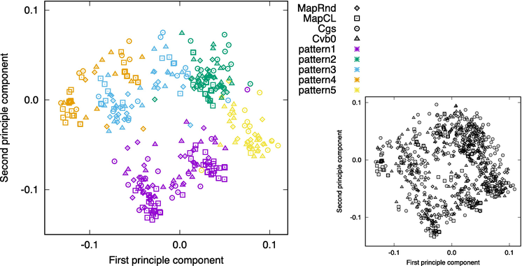
Figure 7 shows a visualization of the solutions using the patterns assigned by the analysis based on word distribution and the coordinate values assigned by the analysis based on topic distribution. Figure 7 (left) is more useful than Figure 7 (right) (equivalent to Figure 3 (top)) in finding a solution, as it provides additional information on the patterns needed in the first step.

The solutions for patterns 1–5 in Figure 7 (left) are grouped together in each pattern. It means that the solutions with the same pattern are also similar to each other in topic distribution. It is interesting to confirm that word and topic distributions are related.

As the experimental results show, analysis using word distribution will play a major role in the search for a solution. This is because the results can be presented in a way that is understandable to humans and can be compared to the objective. Analysis using topic distribution will play the role of a “map” that provides another point of view when a decision is not clear. A map that provides a view of all the solutions should be useful.

6. Conclusion

It has been reported that information-theoretic clustering outperforms spherical clustering when targeting text data [17]. Topic modeling is an extension of information-theoretic clustering (see Appendix A), which is why we apply this technique to document analysis. The solutions obtained through modeling are diverse. In past studies, however, diversity has not been adequately considered. This chapter introduced methods for analyzing diverse solutions and obtaining an overall picture of the solutions. Also, we showed effectiveness of the methods through experiments.

In this study, we found that there are many solutions that are different from each other in topic models. It is difficult to obtain an appropriate solution by chance. Furthermore, problems in the world, not to mention smart cities, are complex and change rapidly, so there is a high risk of missing important topics. The proposed analysis methods should be useful in the search for solutions. There are various extensions of topic models, such as dynamic topic models [21], but even there, a diversity of solutions may exist. The approach presented in this chapter may also be used for analyses using such models.

Acknowledgments

This work was supported by JSPS KAKENHI Grant Number 18 K11442.

References

1.Hofmann T. Unsupervised learning by probabilistic latent semantic analysis. Machine Learning. 2001;42(1–2):117-196
2.Blei DM, Ng AY, Jordan MI. Latent dirichlet allocation. Journal of Machine Learning Research. 2003;3:993-1022
3.Uchiyama T. A method for analyzing solution diversity in topic models. In: Proceedings of 5th International Conference on Business and Industrial Research (ICBIR). New York: IEEE; 2018. pp. 29-34. DOI: 10.1109/ICBIR.2018.8391161
4.Uchiyama T, Hokimoto T. Analysis and visualization of solution diversity about topic model. IEICE Transactions D. 2019;J102-D(10):698-707. DOI: 10.14923/transinfj.2019JDP7017
5.Manning CD, Raghavan P, Schütze H. Introduction to Information Retrieval. Cambridge, England: Cambridge University Press; 2008
6.Torgerson WS. Multidimensional scaling: I theory and method. Psychometrika. 1952;17(4):401-419
7.Uchiyama T, Hokimoto T. A word distribution based analysis of the diverse solution at topic model. IEICE Transactions D. 2022;J105-D(5):405-415. DOI: 10.14923/transinfj.2021JDP7053
8.Gondek D, Hofmann T. Non-redundant data clustering. Knowledge and Information Systems. 2007;12(1):1-24
9.Niu D, Dy JG, Jordan MI. Multiple non-redundant spectral clustering views. In: Proceedings of the 27th International Conference on Machine Learning (ICML-10). Madison, Wisconsin, United States: Omnipress; 2010. pp. 831-838
10.Caruana R, Elhawary M, Nguyen N, Smith C. Meta clustering. In: Proceedings of Sixth International Conference on Data Mining. New York: IEEE; 2006. pp. 107-118
11.Iwata T, Yamada T, Ueda N. Probabilistic latent semantic visualization: Topic model for visualizing documents. In: Proceedings of the 14th ACM SIGKDD International Conference on Knowledge Discovery and Data Mining. New York: ACM; 2008. pp. 363-371
12.Griffiths TL, Steyvers M. Finding scientific topics. In: Proceedings of the National Academy of Sciences. Vol. 101. Washington, D.C.: National Academy of Sciences; 2004. pp. 5228-5235
13.Teh YW, Newman D, Welling M. A collapsed variational Bayesian inference algorithm for latent dirichlet allocation. In: Proceedings of Advances in Neural Information Processing Systems. Cambridge, MA, United States: MIT Press; 2007. pp. 1353-1360
14.Chien JT, Wu MS. Adaptive Bayesian latent semantic analysis. IEEE Transactions on Audio, Speech, and Language Processing. 2008;16(1):198-207
15.Asuncion A, Welling M, Smyth P, Teh YW, Asuncion A, Max W, et al. On smoothing and inference for topic models. In: Proceedings of the Twenty-Fifth Conference on Uncertainty in Artificial Intelligence. Arlington, Virginia, United States: AUAI Press; 2009. pp. 27-34
16.Uchiyama T. Improvement of probablistic latent semantic analysis using information-theoretic clustering. IEICE Transactions D. 2017;J100-D(3):419-426. DOI: 10.14923/transinfj.2016JDP7085
17.Uchiyama T. Information theoretic clustering and algorithms. In: Hokimoto T, editor. Advances in Statistical Methodologies and Their Application to Real Problems. London, UK: IntechOpen; 2017. pp. 93-119. DOI: 10.5772/66588
18.Newman MEJ, Girvan M. Finding and evaluating community structure in networks. Physical Review E. 2004;69(2):026113
19.Dua D, Graff C. UCI Machine Learning Repository. Available from: http://archive.ics.uci.edu/ml/ [Accessed: 16 May 2022]
20.20news-bydate data at Home page for 20 Newsgroups data set. Available from: http://qwone.com/jason/20Newsgroups/20news-bydate-matlab.tgz [Accessed: 16 May 2022]
21.Blei DM, Lafferty JD: Dynamic topic models. In: Proceedings of the 23rd International Conference on Machine Learning. New York: Association for Computing Machinery; 2006. pp. 113–120
Written By
Toshio Uchiyama and Tsukasa Hokimoto
Reviewed: June 21st, 2022Published: July 26th, 2022