Open Access is an initiative that aims to make scientific research freely available to all. To date our community has made over 100 million downloads. It’s based on principles of collaboration, unobstructed discovery, and, most importantly, scientific progression. As PhD students, we found it difficult to access the research we needed, so we decided to create a new Open Access publisher that levels the playing field for scientists across the world. How? By making research easy to access, and puts the academic needs of the researchers before the business interests of publishers.
We are a community of more than 103,000 authors and editors from 3,291 institutions spanning 160 countries, including Nobel Prize winners and some of the world’s most-cited researchers. Publishing on IntechOpen allows authors to earn citations and find new collaborators, meaning more people see your work not only from your own field of study, but from other related fields too.
Fear conditioning is a behavioral paradigm of learning to predict aversive events. It is a form of associative learning that memorizes an undesirable stimulus (e.g., an electrical shock) and a neutral stimulus (e.g., a tone), resulting in a fear response (such as running away) to the originally neutral stimulus. The association of concurrent events is implemented by strengthening the synaptic connection between the neurons. In this paper, with an analogous methodology, we reproduce the classic fear conditioning experiment of rats using mobile robots and a neuromorphic system. In our design, the acceleration from a vibration platform substitutes the undesirable stimulus in rats. Meanwhile, the brightness of light (dark vs. light) is used for a neutral stimulus, which is analogous to the neutral sound in fear conditioning experiments in rats. The brightness of the light is processed with sparse coding in the Intel Loihi chip. The simulation and experimental results demonstrate that our neuromorphic robot successfully, for the first time, reproduces the fear conditioning experiment of rats with a mobile robot. The work exhibits a potential online learning paradigm with no labeled data required. The mobile robot directly memorizes the events by interacting with its surroundings, essentially different from data-driven methods.
Department of Electrical and Computer Engineering, Michigan Tech, USA
Yan Zhang
Department of Biological Sciences, Michigan Tech, USA
Hongyu An*
Department of Electrical and Computer Engineering, Michigan Tech, USA
*Address all correspondence to: hongyua@mtu.edu
1. Introduction
Associative memory learning is a ubiquitous online learning paradigm in animals [1, 2, 3]. Unlike the data-driven learning schemes of current Artificial Intelligence (AI), animals have the capability of memorizing the events that occur at the same time or within a certain time interval. The underlying memorization mechanism in the nervous system is the synaptic connection that becomes strengthened under the stimulus of the firing neurons evoked by concurrent events. The strengthened synaptic connection enables the response neurons at the conditional pathway to receive a larger amount of the synaptic transmitter. As a result, the response neuron in the conditional signal pathway will fire, even though it originally did not become active. In other words, the memorization of the relationship between concurrent events is achieved by signal pathway modification rather than backpropagation. The signal pathway modification is accomplished by synaptic plasticity. An AI system with associative memory potentially provides an alternative way of active self-learning by constantly interacting with environments. The signal pathway modification can be accomplished with a few training processes, leading to less dependence on large-size datasets. For data-driven deep learning, for example, Deep Neural Networks (DNNs), the large datasets prolong training time and increase energy demands. Consequently, the application of deep learning is highly reliant on bulky supercomputers that are not feasible and applicable to scenarios that require Size, Weight, and Power (SWaP) constraints [4, 5]. In addition, massive and labeled data are costly to build or even not practical to collect, such as the Lunar and Martian terrain data [5].
Numerous studies have implemented associative memory with neuromorphic systems [2, 6, 7, 8, 9, 10, 11, 12, 13]. However, these studies merely complete a small-scale association with a few neurons in simulation environments. It is far away from the capability of associative memory learning to enable animals to self-learn and explore independently in an unknown environment. In addition, pretraining processes with labeled datasets are still required for these studies [9, 10, 11, 12, 13]. In order to resolve these limitations of studies on associative learning, we have designed several experiments of associative memory in real-world scenarios using a mobile robot and neuromorphic chips. Our system of associative memory is validated by reproducing one of the classic associative memory learning in rats: fear conditioning. In fear conditioning experiments, the rats learn to associate a particular neutral Conditional Stimulus (CS), for example, tone, with an aversive Unconditional Stimulus (US), such as an electrical foot shock, and show a fear response, freezing or running away. The rats learn fear conditioning after several training sessions and exhibit long-lasting behavioral changes. Several brain regions have been proven to be involved in the learning process, including frontotemporal amygdala, hippocampus, and so on. The process of fear conditioning cannot be reproduced by other state-of-the-art associative memory models [2, 6, 7, 8, 9, 10, 11, 12, 13] due to their limited neural network sizes. The simple neural network models cannot process informative signals, such as visual signals. These informative signals are processed with large-scale neural assemblies rather than simply a few neurons in the brains [14, 15, 16, 17, 18, 19]. To resolve these limitations, in our design, we use large-scale biological plausible neurons to process the visual signals. Specifically, in our system and experimental designs, the mobile robot with sensors serves as the substitute for the rats in fear conditioning experiments. The neuromorphic chip (Intel Loihi) provides a computational platform for the associative memory learning operation. In our experiment, the brightness of a light emulates the visual stimulus, and the vibration signals from the accelerometer mimic the shock signals to the rats. Thus, the vibration signals are the unpleasant stimulus, and light is the neutral stimulus. The movement of the mobile robot emulates the fear response. The perception of the light and the vibration are separately processed within two different neural assemblies. Two neural assemblies connect to the response neuron, which stimulates the movement of the robot, with two signal pathways. One signal pathway with a weak synaptic connection serves as the conditional signal pathway, while another one with a stronger synaptic connection is the unconditional signal pathway. Thanks to the mobile robot providing a platform directly interacting with the environment, we for the first time, to our best knowledge, implement associative memory as real-time online learning with no pretrained procedure. The contributions of this paper are summarized as follows:
Compared to other state-of-the-art works [9, 10, 11, 12, 13], we have implemented associative memory learning with a mobile robot for an online learning scenario using an Intel Loihi chip.
The work reproduces the classic fear conditioning of rats with solid biological rationales from a cellular level (Hebbian learning) to the behavior level (neural assembly).
Aiming signal pathway modification as the neural network training purpose, which is a novel learning paradigm of associative memory learning.
This work aims to develop a novel self-learning paradigm by emulating associative memory learning of animals. Thus, the study is built upon the reverse engineering of brain function. In specific, the large-scale computational models of associative memory learning are implemented by a neuromorphic system. In this section, we first introduce the state-of-the-art development of neuromorphic computing and systems. Then, the mechanism of associative memory learning at both macroscopic and microscopic levels is analyzed.
2.1 Neuromorphic system
A neuromorphic system emulates nervous systems, such as human brains, aiming at implementing Artificial Intelligence [20, 21, 22, 23, 24, 25]. Human brains have the capability of executing sophisticated missions in unbelievably ultra-low energy. The average power of human brains is as small as ∼20 watts [1]. In addition, unlike the training process required for Artificial Neural Networks (ANNs) using big data, the nervous systems can adjust their responses by constantly interacting with their surroundings. This learning process is referred to as associative memory learning [1]. These incredible capabilities of nervous systems are attributed to their parallelization, high degree of connectivity, adjustable network topology, the colocation of data memory computation, and spike-based information representation.
Human brains consist of billions of neurons and trillions of synapses forming a high-degree and three-dimensional neural network. Through this extraordinarily complex network, an individual neuron can communicate with more than ten thousand other neurons simultaneously. Within this complex neural network, neurons are mainly signal-processing units, and the synapse between neurons connects organs. As computing units, the neurons integrate the received spiking signals in their cell body and send another sequence of spiking signals to other neurons through synapses. The signal strength received by other neurons is depended on the connection strength of the synapses. The connection strength among neurons can be adjusted. This feature is named as synaptic plasticity [1, 26, 27]. In specific, the connection strength among neurons becomes strong if the presynaptic neuron and postsynaptic neuron fire together. This synaptic connection strength change inspired a learning paradigm known as Hebbian learning [28, 29, 30, 31].
In addition, the computational units (neurons) and the memory units (synapses) are located in close proximity. This structure eliminates one of the biggest inefficiencies in the von Neumann architecture that separates computing units and memory at different locations. The physical separation leads to data needing to be constantly transferred back and forth between memory and central processing units (CPUs). Furthermore, neuromorphic systems use sparse and event-based computation, meaning that only a small percentage of the available computing resources are active for a given task, and they are only activated and consuming power as needed in response to present events. Neuromorphic computing attempts to exploit these useful properties by modeling the architecture, neuron and synaptic cells, and the way of learning observed in the brain, enabling a new era of computers and AI [32].
Neuromorphic systems utilize specialized neuromorphic chips with artificial neurons. These chips are generally used to operate spiking neural networks (SNNs), which encode the information with a sequence of spikes just like nervous systems. In an SNN, neurons communicate with each other with discrete “spike” signals. There are various types of neuromorphic chips, such as Intel’s Loihi [33, 34]. Unlike traditional GPUs and CPUs built upon the von Neumann architecture operating on digital information, Loihi chips are specifically designed for neuromorphic computing and asynchronous SNNs. To date, two generations of Loihi chips have been released. The first generation of Loihi chip was revealed in 2017 [33, 34]. Loihi-1 chips consist of 130,000 electronic neurons and 130 million synapses at 128 neuromorphic cores. The advanced 14 nm process of Intel renders the area of the Loihi-1 chip as small as 60 mm2. Loihi-1 chips implement the digital leaky-and-fire neurons located on 128 cores. At each core, the communication among neurons is organized in a mesh configuration. The synapses in Loihi-1 chips are fully configurable and further support weight-sharing and compression features. The plasticity of synapses can be manipulated with various biologically plausible learning rules, such as Hebbian rules, STDP, and reward-modulated rules [33, 34]. The firing behavior of neurons in Loihi chips is implemented when received spikes accumulate to a threshold value in a certain time; the neurons will fire off their own spikes to their connected neurons.
Loihi-1 chips are offered with several neuromorphic platforms providing distinct interfaces for integrating the Loihi-1 chip with other computer systems or Field-Programmable Gate Array (FPGA) devices. Kapoho bay includes 1–2 Loihi chips with a USB interface. Nahuku is a 32-chip Loihi board with a standard FPGA Mezzanine Card (FMC) connector. The FMC connector allows the Nahuku system to communicate with the Arria FPGA development board. Pohoiki Spring is a large-scale Loihi chip with 100 million neurons equipped as a server for remote access. The second generation of the Loihi chips, namely Loihi-2, was introduced in late 2021 [35]. Loihi-2 is fabricated in Intel 4 process, previously referred to as 7 nm technology. Powered by this advanced technology, the area of the Loihi-2 has been reduced to 31 mm2 from 60 mm2 of the first generation Loihi chips. Unlike the rigid neuron models in the last generation of Loihi chips, Loihi-2 realizes fully programmable neuron models. In Loihi-2, the specific behavior of the neurons can be programmed with microcode instructions. The microcode instructions support basic bitwise and math operations that can be used to specify custom neuron models. The Loihi-2 chip is dedicatedly designed for neuromorphic computing and edge devices with parallel computations, achieving high computational and energy efficiency. The comparison between two generations of Loihi chips is summarized in Table 1.
Animals have the capability of memorizing different events if they occur at the same time or with a small time lag. The capability is referred to as associative memory [1]. Associative memory learning was first studied by Ivan Pavlov in the 1890s when he was studying salivation reflex actions in dogs [1]. During Pavlov’s experiments, the dogs originally had a salivation reflex to the presence of food, instead of the sound of whistles. However, if these two signals were presented together several times, the dogs salivated even if they only listened to the sound of a whistle with no food provided. This means the dogs can memorize the sound of whistles as a sign of food [1, 6, 36] through a learning/memorizing process. Through a series of experiments, Pavlov concluded that dogs have the capability of associating two originally irrelevant signals together through a training process, which is referred to as associative memory learning later. In general, two types of stimuli exist in associative memory learning: unconditional stimuli (US) and conditional stimuli (CS). The unconditional stimuli evoke the response with no training required. On the contrary, conditional stimuli demand an associative learning process to acquire corresponding reactions. For instance, in Pavlov’s experiments, the presence of food was the unconditional stimulus, and the sound of whistles was a conditional stimulus (CS). After dogs, further studies have demonstrated that associative memory learning is a self-learning paradigm of a large variety of animals such as rats, bats, and sea slugs [1].
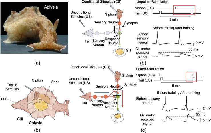
The studies in neuroscience exhibit that signal pathway modification and synaptic plasticity are highly related to associative memory learning [1, 22]. In a nervous system, the shapes of the spiking signals are almost identical (spikes), whether the signals come from the sensation of light or hearing. Thus, neuroscientists hypothesize that brains distinguish these signals by the signal pathways they are traveling to rather than their shapes. This hypothesis is much more straightforward in invertebrates that have simple nervous systems. Figure 1 illustrates part of the nervous system of Aplysia that has two signal pathways from siphon to the gill and from tail to the gill, separately.
Figure 1.
Illustration of associative memory learning of Aplysia.
With these two signal pathways, Aplysia can accomplish a simple version of associative memory learning by memorizing the touch on the tail and stimulus from the siphon. When the tail of an Aplysia is touched, its gill shrinks, demonstrating an unconditional signal pathway. On the contrary, the gill does not shrink if the siphon is cut, exhibiting a conditional signal pathway. By applying a touch to the tail and stimulus on the siphon at the same time several times, the gill motor neuron becomes more responsive to the touch on the siphon alone. At the cellular level, the concurrent stimuli on the siphon and tail lead to a spiking signal overlapping when the stimuli are applied at the same time, shown in Figure 1. As a result, the synaptic connection among neurons, from the siphon to the gill, becomes stronger than the original state. This means the signal pathway from the siphon to the gill becomes unimpeded from blocked. These experiments on Aplysia demonstrate two critical factors for associative memory learning: (1) signal pathway modification and (2) synaptic plasticity.
For more complicated animals, such as rats, the sensation signals are processed not in individual neurons but in a group of neurons. These groups of neurons are referred to as neural assemblies [29, 37, 38, 39]. For example, fear conditioning experiments in rats involve two types of stimuli: electric shock on the food and a sound as neutral stimuli. These two types of signals are processed at different neural regions: auditory thalamus and somatosensory thalamus. The experimental goal is to let the rats associate the neutral sound with undesired electric shock by applying these two stimuli at the same time. Thus, it is one type of associative memory learning scheme. The studies have strong experimental evidence showing that signal pathway modification potentially occurs in lateral nucleus because the output signals from the auditory thalamus and somatosensory thalamus converge at the lateral nucleus [1]. This hypothesizes that associative memory learning in higher animals is accomplished via the association of two, or several, neural assemblies together rather than individual neurons.
3. Reproducing fear conditioning using mobile robots
In this section, we introduce our experimental design for reproducing fear conditioning using mobile robots. In specific, we select visual signals, the brightness of light as the conditional stimulus, and vibration signals as the unconditional stimulus. Vibration signals emulate electric shock applied on the foot of rats in fear conditioning experiments, while light signals serve as a neutral stimulus. We select the Leaky Integrate and Fire (LIF) neuron model to build neural assemblies for both UC and CS signal pathways due to its simplicity. In our experiments, the Nengo simulator has been used to implement the system [40]. Our mobile robot is controlled with the Robot Operating System (ROS) [41].
3.1 Neuron model
In our experiment, a mobile robot is placed on a vibration platform and unconditionally responds to the acceleration signals, which will be detected with an inertial measurement unit (IMU). The acceleration signals emulate the unpleasant stimulus in the fear conditioning experiment in rats. The conditional stimulus is mimicked with the brightness of a light. Two neural assemblies will be built for processing these UC and CS signals. At last, the movement of a mobile robot is controlled by the motion neurons. We design several specific neurons for precepting the brightness of lights, detecting vibrations, and controlling mobile robots. All these neurons are customized from classic Leaky Integrate and Fire (LIF) neurons, which are characterized using the following eqs. [42]:
CmdVmdt=GLEL−Vm+A∗Iapp,
ifVm>VththenVm=Vreset,E1
τRC=Cm/GL,E2
where Cm is the membrane capacitance, Vm is the membrane potential, GLis the leak conductance, A is the input signal gain, ELis the leak potential, Iapp is the input current, and τRC is the RC time constant. The specific values of these parameters in our design are summarized in Table 2.
For all the neurons in Table 2, the membrane potential is fixed at 1 V, and input gain is modified instead. They all use the Nengo LIF model’s default τRC of 0.02 seconds because it is sufficient for our desired functionality. The other two parameters are calculated and optimized based on our experimental setups so that they can produce the desired responses for their respective uses. In specific, for the vibration detection neuron, gain (A) and bias (Vreset) are empirically derived so that it fires with vibration stimulus input instead of a small sudden move. The movement response neuron is a typical LIF configured to spike whenever it receives any sustained input spikes, either from vibration neurons or from brightness neurons. The brightness neuron is the Layer 3 neuron in Table 3 and is a LIF neuron with empirically derived gain and bias so that it fires only when the Light Feature neurons have a high enough collective output. More details regarding how these neurons work will be introduced in subsequent sections.
Neuron types
τRC
A
Vreset (V)
Vth(V)
Vibration neuron
0.02
1.3
0.6
1.0
Brightness neuron
0.02
0.3
−1.0
1.0
Movement neuron
0.02
1.0
0.01
1.0
Table 2.
LIF neuron parameters.
LCA neuron layer
τRC(s)
A
Vreset (V)
Vth (V)
Layer 2
∞
1.0
-λ = 0.85
1.0
Layer 3
0.02
0.3
−1.0
1.0
Table 3
LCA neuron parameters in layers 2 and 3.
3.2 Vibration perception
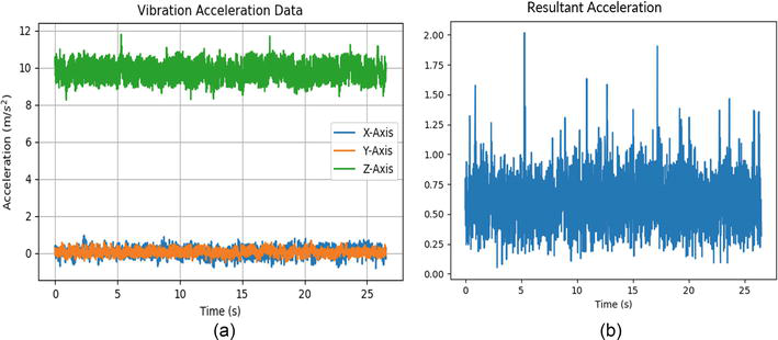
The accelerometer within the onboard IMU of the mobile robot is used to measure the acceleration. In our experiment design, acceleration is used for evaluating the degree of vibration. Our vibration platform generates vibration signals with 1.2 mm amplitude at 25 Hz. In general, the IMU measures three-dimensional accelerations from x, y, and z directions as shown in Figure 2a. In Figure 2a, the acceleration in the z-axis (vertical) has the largest magnitude as it includes the intrinsic gravity of the earth (9.8 m/s2). Because the mobile robot should only count the acceleration from the vibration platform, the gravity effect is removed from z-direction by subtracting the standard gravity (9.8 m/s2). Thus, the resultant acceleration, which is used for evaluating the vibration states, is calculated by the equation:
Figure 2.
(a) Acceleration data of IMU for three dimensions denoted as X-axis (blue), Y-axis (orange), and Z-axis (green). (b) Resultant acceleration.
ares=ax2+ay2+az−9.82,E3
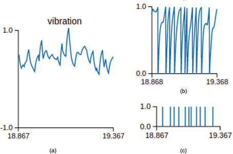
where ares is the resultant acceleration and ax, ay, andaz are the accelerations in X-axis, Y-axis, and Z-axis, respectively. The resultant acceleration measured by our mobile robot is depicted in Figure 2b. The resultant acceleration is imported into the vibration detection neuron. A vibration detection neuron, implemented with LIF, is connected to the accelerometer, and it fires if the detected acceleration is larger than its threshold (shown in Figure 3). At last, a movement neuron is specifically designed to control our mobile robot moving away from the vibration platform with specific direction and speed. The motion neuron is also implemented by a LIF neuron. The parameters of motion neuron are listed in Table 2. The active motion neuron will trigger a specific movement (escape) response that commands the mobile robot to move away from the vibration platform at a speed of 0.3 m/s.
Figure 3.
Vibration detection neuron response to the acceleration input: (a) input vibration signals; (b) membrane potential of the vibration detection neuron; (c) output spiking signals of the vibration detection neuron.
3.3 Visual perception with sparse coding and locally competitive algorithm
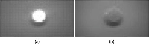
In order to process visual stimuli, we designed an artificial neural network (ANN) to activate the output neuron if the light is on. Figure 4 illustrates the brightness of the light captured by the stereo camera equipped with our mobile robot. The stream of visual signals captured by the camera is sent to the computer via ROS. As the images arrive, their resolution is 24x48 pixels, and the pixel brightness is normalized to the range between −1 and 1.
Figure 4.
Sights of the light off and on.
An ANN model based on 2D sparse coding is used for detecting the brightness of lights to further determine whether the light is on or off. The goal of sparse coding is to represent an input vector with a linear combination of features from a dictionary. This can be modeled by the LASSO optimization function:
E=12x−Φ·a22+λ·a1,E4
a∗=argminaEa,E5
where the features Φi are columns of the dictionary matrix Φ, and the sparse code a⃰ is the set of coefficients ai for which the reconstruction (Φ·a) of the input x minimizes the cost (E). The sparsity penalty λ reduces the amount of non-zero terms in a by penalizing its 1-norm.
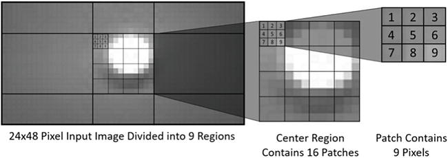
Typically, the sparse code a⃰ is used to reconstruct x or as the input to a classifier. In 2D image sparse coding, we divided the image into patches the size of the features Φj. Thus, each patch is a sparse-coding optimization problem. As shown in Figure 5, the light image is divided into 9 sub-regions, which are further partitioned into patches. The Spiking Locally Competitive Algorithm (LCA) model [43] is used to solve Eq. (6) and Eq. (7):
Figure 5.
Image region layout and patch structure.
u̇=1τΦTx−u−ΦTϕ−I·a,a=TλuE6
Tλu=0ifu≤λ,elseTλu=u−λE7
where ai is the firing rate of neuron i, ui is the average soma current, τ is the discrete time step, and Tλ is the thresholding function that determines if neuron i will fire.
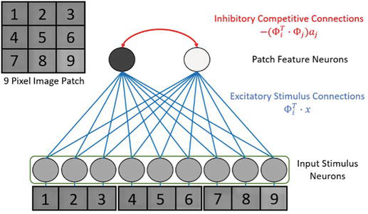
Figure 6 illustrates a spiking LCA network for solving one image patch (Figure 5). The model consists of the first layer for the input x and the second layer for the sparse code a∗. The firing rates of each neuron are the coefficients ai. The neurons in the second layer are referred to as feature neurons as each of them is associated with one feature Φi. Typically, an overcomplete dictionary is used in sparse coding, resulting in a having a larger size than x. Our model represents each patch with only two features, light and dark. Thus, the dictionary in Figure 6 only contains two features. The dictionary could be made complete by having more feature neurons than the size of x, 9 in this case. There could be copies or variations of light and dark features to make the dictionary overcomplete.
Figure 6.
LCA network for one patch including input neurons (Layer 1) and path neurons (Layer 2).
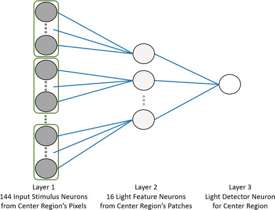
The convolutional stride between the image patches is equal to the width of one patch (3 pixels), resulting in no overlap between them. This simplifies the LCA model by removing connections between feature neurons in overlapping patches. The neural network contains a third layer with one neuron for each of the 9 regions in the image as illustrated in Figure 7. The third layer has one neuron as an output neuron integrating the light feature neurons of every patch. In Figure 7, each neuron at layer 1 simply has a firing rate proportional to the pixel intensity it represents, serving as a spike generator. The neurons at layer 2 and layer 3 are Integrate and Fire neurons with the parameters listed in Table 3. The layer 2 neurons are the LCA neurons in a single-layer LCA configuration. The parameters of the Integrate and Fire LCA feature neuron in layer 2 are implemented via the Vreset parameter, which was empirically adjusted until the desired response was achieved from the feature neurons. The other parameters are assigned according to the LCA model [43]. The neurons in layer 3 have the parameters derived for brightness neurons from Table 2.
Figure 7.
Neural network for light detection in the center region. Note: The dark feature neurons in Layer 2 are not shown.
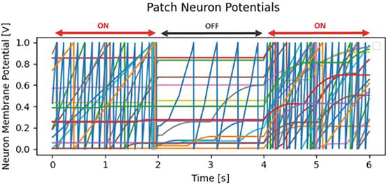
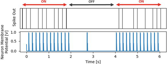
When the high brightness signals of the light (Figure 4a) enter the network, the light feature neurons in the center patches start to fire. The light-off image (Figure 4b) subsequently reduces the activity in the neurons. These images are alternately presented as inputs, shown in Figure 8. This causes the neurons in layer 3 to fire for the center region from the time periods 0 s to 2 s and 4 s to 6 s, as shown in Figure 9. Those are the times the light is on in our experiment.
Figure 8.
Membrane potential of light feature neurons (Layer 2) in center region image patches.
Figure 9.
Spiking signals of Layer 3 neuron.
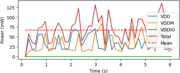
The sparse coding network operates at Intel Loihi neuromorphic chip for power and energy estimation. Our associative memory neural networks are implemented with Nengo simulator and further deployed into Loihi chips by Intel’s NxSDK as a backend [44]. The NxSDK contains a built-in LCA network implementation, which can be connected to the rest of the SNN. The parameters from Table 3 were used to create the same LCA network from Nengo for deployment on Loihi. In the Loihi chip, the synaptic weights only have a 4-bit resolution, instead of a 24-bit resolution in typical computational platforms. Thus, the time of one simulation is reduced from 1 ms to 20 ms at the Loihi platform. The measured powers are shown in Figure 10. The average VDD power is 30 mW, and the average VDDM power is 29 mW. In Figure 10, the VDDIO has a relatively negligible contribution to the total power, while VDD and VDDM have effectively equal contributions. The power is measured and reported with the average consumption across every 8 timesteps while the experiment is under operation.
Figure 10.
Power consumption for sparse coding network with the Loihi chip. The VDD represents the compute logic; VDDM is the SRAMs, and VDDIO is the IO interface.
3.4 Associative memory learning experiment and results
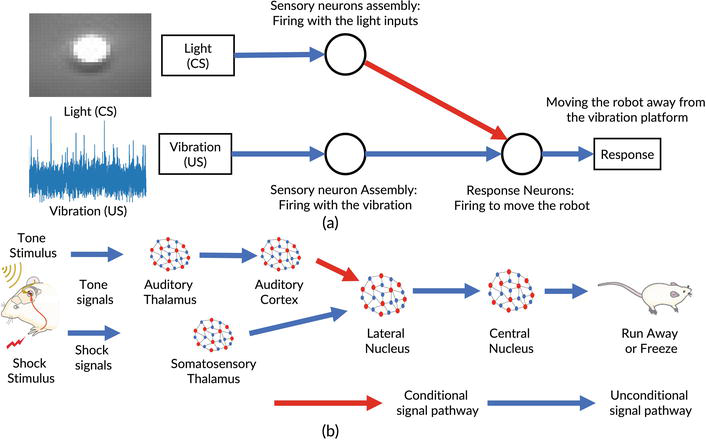
Figure 11 illustrates the comparison of signal pathway modification between our SLN system and fear conditioning of rats. In our design, the brightness signal from light serves as a conditional stimulus, and the acceleration from the vibration platform is the unconditional stimulus. These two signals emulate the electric shock and sound signals in fear conditioning experiments. The movement of our mobile robot away from the vibration platform emulates the fear response of rats. The red arrows (Figure 11) represent the weak synaptic connections in the conditional signal pathway, while the blue arrows represent the unconditional pathway with weaker synaptic connections. During associative memory learning, the synaptic connection (red arrow) will be strengthened by Hebbian learning.
Figure 11.
(a) Our SLN system for associative memory learning implementation. (b) Fear conditioning in rats.
In the brains of rats, shock signals and tone signals are processed at different neural regions: auditory thalamus and somatosensory thalamus. The output signals from these two regions converge at lateral nucleus [1]. Originally, the rat has no fear reaction to a neutral tone. However, when the tone is presented with a foot shock associated with tone signals, the rat starts memorizing the relationship between the tone and the shock. After multiple times, the tone alone will stimulate a fear response, indicating the accomplishment of the associative memory learning [1].
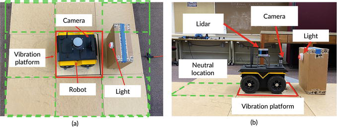
Our experimental setup to emulate fear conditioning using our mobile robot is shown in Figure 12. The mobile robot is placed on a testing platform, which is constructed with 9 wooden boxes. The dimension of each box is 23 in (L) × 23 in (W) × 8 in (H). A vibration plate is installed underneath the center platform, which is marked in red square in Figure 12a. The vibration plate can provide vibration signals (15–40 Hz) emulating an unpleasant stimulus (the electrical shock) in fear learning on the rats. The other eight platforms with no installed vibration plate are marked in green-dashed squares in Figure 12.
Figure 12.
Fear conditioning imitation experimental setup with the mobile robot: (a) top view; (b) side view.
For the fear response, the robot is expected to move away from the vibration platform to the neutral location if unpleasant stimuli, such as vibration, are applied. The specific experimental procedures aiming to reproduce the experimental process of rats in fear conditioning are:
Turn on the light, expecting no response (testing conditional signal pathway).
Turn on the vibration platform, and the robot moves (testing the unconditional signal pathway).
Reset the robot position.
Turn on the light, and then turn on the vibration platform; the robot moves (conducting the associative memory learning process such that the conditional and unconditional stimuli are provided at the same time).
Reset the robot position.
Turn on the light alone, and the robot moves, indicating that associative memory learning is accomplished successfully.
The synaptic weights are modified based on Hebbian learning [42, 45]. Hebbian learning states that when the pre- and postsynaptic neurons are both active at the same time, the synaptic weights between them will be modified using the eqs. [42, 45]:
w=ηrirj,E8
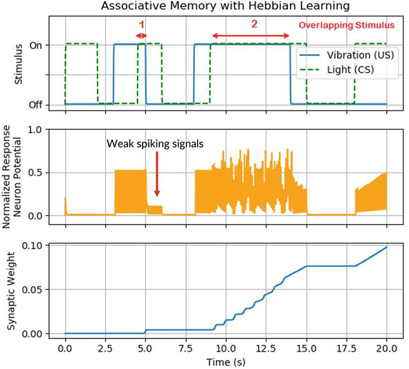
where the ri and rj are firing rates of pre- and postsynaptic neurons, respectively, and the η is the learning rate, determining the changing rate of synaptic weight. In our experiment, the learning rate η is 2×10⁻⁴. Figure 13 shows that the initial synaptic weights between the brightness detection neuron (CS) and the movement neuron are small. Consequently, the brightness stimulus of the light cannot be delivered to the movement neuron to stimulate it to fire. As a result, the synaptic weights between the brightness detection neuron and movement neuron stay constant. When the vibration (US) is applied to the vibration detection neuron, the movement neuron starts to fire. When the vibration and light are applied to the system, both the brightness detection neuron and the movement neuron are active, resulting in the synaptic weight’s increase. Figure 13 illustrates that the synaptic weights increase when the vibration and light stimuli are both applied. However, the first overlapping time frame is not long enough to establish a significant synaptic weight modification. Thus, a sequence of weak spiking signals is observed from the response neuron after the vibration is removed, which is marked in Figure 13. In contrast, the second overlapping period is longer than the first one, which leads to a larger increase in synaptic weights. Thereby, after learning, the response neuron (movement detection neuron) will fire with a visual stimulus (light) even with no vibration stimulus. This demonstrates an accomplishment of associative memory learning.
Figure 13.
Change of synaptic weight during associative memory learning.
In the experiments, the synaptic weights between the brightness detection neuron and the movement neuron are modified during the training process. As a result, after associative memory learning, the mobile robot will move away from the vibration platform under the stimulus of light, even with no vibration signal presented, demonstrating successful online learning in real-time. Compared to other state-of-the-art associative memory works listed in Table 4, we reproduce the classic fear conditioning experiments of rats using a mobile robot and the Loihi chip rather than simply simulation. In addition, the scales of our neural networks outperform other works.
In this paper, we implement a classic self-learning paradigm in rats: associative memory learning (fear conditioning) using a mobile robot and a neuromorphic system (Loihi chip) in an online learning scenario. In specific, we use a mobile robot as the substitute for the rats in fear conditioning experiments. Two signal pathways are assigned for conditional and unconditional stimuli. In our experiments, vibration signals emulate unconditional stimuli, while brightness of lights is assigned as conditional stimuli. Originally, the mobile robot only moves when it detects vibration signals. After providing these two signals at the same time several times, the robot performs a movement when light signals are present alone. The detections of lights and vibrations are implemented with Integrate and Fire Neurons. In addition, the movement of the robot is controlled by the specific-designed response neurons. The signal pathway modification during associative memory learning is implemented with Hebbian learning. Compared to other state-of-the-art works, our work successfully reproduces the fear conditioning of rats in a real-world scenario with no labeled data and pretraining process.
As Intel Neuromorphic Research Community (INRC) members, the authors would like to thank Intel Labs for providing the neuromorphic Loihi chips for our online learning studies.
References
1.Kandel ER, Schwartz JH, Jessell TM, Siegelbaum SA, Hudspeth A. Principles of Neural Science. New York: McGraw-Hill; 2000
2.Sun J, Han G, Zeng Z, Wang Y. Memristor-based neural network circuit of full-function pavlov associative memory with time delay and variable learning rate. In: IEEE Transactions on Cybernetics. New York, USA: IEEE; 2019
3.Kohonen T. Self-Organization and Associative Memory. New York, USA: Springer Science & Business Media; 2012
4.Goodfellow I, Yoshua B, Aaron C. Deep learning. Learning. 2016;2016:785. DOI: 10.1016/B978-0-12-391420-0.09987-X
5.Devlin J, Chang M.-W., Lee K, Toutanova K. Bert: Pre-training of deep bidirectional transformers for language understanding. arXiv preprint arXiv:1810.04805. 2018
6.An H, An Q, Yi Y. Realizing behavior level associative memory learning through three-dimensional memristor-based neuromorphic circuits. In: IEEE Transactions on Emerging Topics in Computational Intelligence. New York, USA: IEEE; 2019
7.Hu SG et al. Associative memory realized by a reconfigurable memristive Hopfield neural network. Nature Communications. 2015;6:1-5. DOI: 10.1038/ncomms8522
8.Moon K et al. Hardware implementation of associative memory characteristics with analogue-type resistive-switching device. Nanotechnology. 2014;25:(49). DOI: 10.1088/0957-4484/25/49/495204
9.Yang J, Wang L, Wang Y, Guo T. A novel memristive Hopfield neural network with application in associative memory. Neurocomputing. 2017;227:142-148. DOI: 10.1016/j.neucom.2016.07.065
10.Liu X, Zeng Z, Wen S. Implementation of memristive neural network with full-function pavlov associative memory. IEEE Transactions on Circuits and Systems I: Regular Papers. 2016;63(9):1454-1463
11.Hu X, Duan S, Chen G, Chen L. Modeling affections with memristor-based associative memory neural networks. Neurocomputing. 2017;223:129-137. DOI: 10.1016/j.neucom.2016.10.028
12.Moon K et al. Hardware implementation of associative memory characteristics with analogue-type resistive-switching device. Nanotechnology. 2014;25(49):495204
13.Eryilmaz SB et al. Brain-like associative learning using a nanoscale non-volatile phase change synaptic device array. Frontiers in Neuroscience Switzerland. 2014;8. Available from: https://www.frontiersin.org/articles/10.3389/fnins.2014.00205/full
14.Roy DS et al. Brain-wide mapping reveals that engrams for a single memory are distributed across multiple brain regions. Nature Communications. 2022;13(1):1-16
15.Josselyn SA, Tonegawa S. Memory engrams: Recalling the past and imagining the future. Science. 2020;367(6473):eaaw4325
16.Nomura H, Teshirogi C, Nakayama D, Minami M, Ikegaya Y. Prior observation of fear learning enhances subsequent self-experienced fear learning with an overlapping neuronal ensemble in the dorsal hippocampus. Molecular Brain. 2019;12(1):1-8
17.DeNardo LA et al. Temporal evolution of cortical ensembles promoting remote memory retrieval. Nature Neuroscience. 2019;22(3):460-469
18.Khalaf O, Resch S, Dixsaut L, Gorden V, Glauser L, Gräff J. Reactivation of recall-induced neurons contributes to remote fear memory attenuation. Science. 2018;360(6394):1239-1242
19.Kitamura T et al. Engrams and circuits crucial for systems consolidation of a memory. Science. 2017;356(6333):73-78
20.Mead C. Neuromorphic electronic systems. Proceedings of IEEE. 1990;78(10):1629-1636
21.Roy K, Jaiswal A, Panda P. Towards spike-based machine intelligence with neuromorphic computing. Nature. 2019;575(7784):607-617
22.Zins N, Zhang Y, Yu C, An H. Neuromorphic computing: A path to artificial intelligence through emulating human brains. In: Frontiers of Quality Electronic Design. New York, USA: Springer; 2023. pp. 259-296
23.An H. Powering Next-Generation Artificial Intelligence by Designing Three-Dimensional High-Performance Neuromorphic Computing System with Memristors. DriveBlacksburg, VA: Virginia Tech; 2020
24.Bai K, Yi Y. Opening the “Black Box” of Silicon Chip Design in Neuromorphic Computing in Bio-Inspired Technology. London, UK: IntechOpen; 2019
25.Bai K, Yi Y. DFR: An energy-efficient Analog delay feedback reservoir computing system for brain-inspired computing. ACM Journal on Emerging Technologies in Computing Systems (JETC). 2018;14(4):45
26.Baird E, Srinivasan MV, Zhang S, Cowling A. Visual control of flight speed in honeybees. Journal of Experimental Biology. 2005;208(20):3895-3905
27.Kern R, Boeddeker N, Dittmar L, Egelhaaf M. Blowfly flight characteristics are shaped by environmental features and controlled by optic flow information. Journal of Experimental Biology. 2012;215(14):2501-2514
28.Kempter R, Gerstner W, Van Hemmen JL. Hebbian learning and spiking neurons. Physical Review E. 1999;59:4498-4514. DOI: 10.1103/PhysRevE.59.4498
29.Levy N, Horn D, Meilijson I, Ruppin E. Distributed synchrony of spiking neurons in a Hebbian cell assembly. Advances in Neural Information Processing Systems. 2000;14:129-135
30.Van Rossum MC, Bi GQ, Turrigiano GG. Stable Hebbian learning from spike timing-dependent plasticity. Journal of Neuroscience. 2000;20(23):8812-8821
31.Caporale N, Dan Y. Spike timing–dependent plasticity: A Hebbian learning rule. Annual Review of Neuroscience. 2008;31:25-46
32.Bai K, An Q, Yi Y. Deep-DFR: A memristive deep delayed feedback reservoir computing system with hybrid neural network topology. In: Proceedings of the 56th Annual Design Automation Conference 2019. New York, USA: ACM; 2019. p. 54
33.Davies M et al. Advancing neuromorphic computing with Loihi: A survey of results and outlook. Proceedings of IEEE. 2021;109(5):911-934
34.Davies M et al. Loihi: A neuromorphic manycore processor with on-chip learning. IEEE Micro. 2018;38(1):82-99
35.Orchard G et al. Efficient neuromorphic signal processing with loihi 2. In: 2021 IEEE Workshop on Signal Processing Systems (SiPS). New York, USA: IEEE; 2021. pp. 254-259
36.Pavlov PI. Conditioned reflexes: An investigation of the physiological activity of the cerebral cortex. Annals of Neurosciences. 2010;17(3):136. DOI: 10.5214/ans.0972-7531.1017309
37.Lansner A. Associative memory models: From the cell-assembly theory to biophysically detailed cortex simulations. Trends in Neurosciences. 2009;32(3):178-186
38.Snider GS. Self-organized computation with unreliable, memristive nanodevices. Nanotechnology. 2007;18. DOI: 10.1088/0957-4484/18/36/365202
39.Greig WJ. Integrated circuit packaging, assembly and interconnections. Integrated Circuit Packaging, Assembly and Interconnections. 2007;2007:1-296. DOI: 10.1007/0-387-33913-2
40.Bekolay T et al. Nengo: A Python tool for building large-scale functional brain models. Frontiers in Neuroinformatics. 2014;7:48
41.DiLuoffo V, Michalson WR, Sunar B. Robot operating system 2: The need for a holistic security approach to robotic architectures. International Journal of Advanced Robotic Systems. 2018;15(3):172
42.Miller P. An Introductory Course in Computational Neuroscience. Cambridge, MA: MIT Press; 2018
43.Tang PTP, Lin T.-H, Davies M. Sparse coding by spiking neural networks: Convergence theory and computational results. arXiv preprint arXiv:1705.05475. 2017
44.Rueckauer B, Bybee C, Goettsche R, Singh Y, Mishra J, Wild A. NxTF: An API and compiler for deep spiking neural networks on Intel Loihi. ACM Journal on Emerging Technologies in Computing Systems (JETC). 2022;18(3):1-22
45.Dayan P, Abbott LF. Theoretical neuroscience: computational and mathematical modeling of neural systems. Computational Neuroscience Series. 2001;2001:281-328
46.Ziegler M et al. An electronic version of Pavlov's dog. Advanced Functional Materials. 2012;22(13):2744-2749. DOI: 10.1002/adfm.201200244
47.Pershin YV, Di Ventra M. Experimental demonstration of associative memory with memristive neural networks. Neural Networks. 2010;23(7):881-886
48.An H, Zhou Z, Yi Y. Memristor-based 3D neuromorphic computing system and its application to associative memory learning. In: 2017 IEEE 17th International Conference on Nanotechnology, NANO 2017. New York, USA: IEEE; 2017. pp. 555-560. DOI: 10.1109/NANO.2017.8117459
Written By
Noah Zins, Yan Zhang and Hongyu An
Submitted: January 20th, 2023Reviewed: February 3rd, 2023Published: February 24th, 2023