Open Access is an initiative that aims to make scientific research freely available to all. To date our community has made over 100 million downloads. It’s based on principles of collaboration, unobstructed discovery, and, most importantly, scientific progression. As PhD students, we found it difficult to access the research we needed, so we decided to create a new Open Access publisher that levels the playing field for scientists across the world. How? By making research easy to access, and puts the academic needs of the researchers before the business interests of publishers.
We are a community of more than 103,000 authors and editors from 3,291 institutions spanning 160 countries, including Nobel Prize winners and some of the world’s most-cited researchers. Publishing on IntechOpen allows authors to earn citations and find new collaborators, meaning more people see your work not only from your own field of study, but from other related fields too.
There is an increasing demand for the performance optimization under the reliability constraints in various engineering problems. These problems are commonly known as reliability-based design optimization (RBDO) problems. Among different RBDO frameworks, the decoupled methods are widely accepted for their high efficiency and stability. However, when facing problems with high nonlinearity and nonnormally distributed random variables, they lose their computational performance. In this study, a new efficient decoupled method with two level quantile-based sampling strategy is presented. The strategies introduced for two level sampling followed by information reuse of nearby designs are intended to enhance the sampling from failure region, thus reducing the number of samples to improve the efficiency of sampling-based methods. Compared with the existing methods which decouples RBDO in the design space and thus need to struggle with searching for most probable point (MPP), the proposed method decouples RBDO in the probability space to further make beneficial use of an efficient optimal shifting value search strategy to reach an optimal design in less iterations. By comparing the proposed method with crude MCS and other sampling-based methods through benchmark examples, our proposed method proved to be competitive in dramatically saving the computational cost.
School of Computer Science and Statistics, Trinity College Dublin, Ireland
Elyas Fadakar
Electronics and Information Engineering, Beihang University (BUAA), China
Masoud Ebrahimi*
Faculty of Mechanical Engineering, Tarbiat Modares University, Iran
*Address all correspondence to: ebrahimikm@modares.ac.ir
1. Introduction
It is a high priority for the engineers to reach an optimal design scheme for the entire system. However, optimality alone cannot guarantee the reliability of the design since theoretically, the optimal design solutions are very close to the boundaries of the reliability constraints. So, the optimal solution in practice can be very sensitive to the design uncertainties and may easily crosses the reliability constraint limits. To avoid such a situation, the optimal design should either be represented with a confidence range (margin) or an optimization process with the objective of maintaining the desired level of reliability [1]. Reliability-based design optimization (RBDO) methodologies have been introduced to incorporate uncertainties in the design components and to provide a scheme seeking an optimal solution with the desired level of reliability.
To better understand the mechanism of these methods, researchers divided them into three major categories [2]:
Double-loop strategies: This model is not very efficient as it accommodates nested optimization loops where the inner loop is the reliability analysis and the outer loop runs the main deterministic design optimization (DDO) problem subject to the reliability requirements [3]. The computational inefficiency lies in the fact that each constraint is under the reliability analysis even if it is very far from the deterministic optimal point and thus has a confidence level (probability of success) very close to 1 [4].
Decoupled strategies: If the reliability analysis is not called at every cycle of the main optimization, it is classified as a decoupled strategy [5].
Unilevel methods: It replaces the inner reliability analysis by Karush–Kuhn–Tucker (KKT) optimality conditions on the optimum point and then enforces it as a constraint itself in the main design optimization loop [2, 5, 6, 7].
Single loop methods: This approach arranges the reliability analysis and DDO in a sequential manner so that in each cycle, the probabilistic constraints are transformed into equivalent deterministic constraints [8, 9, 10, 11, 12, 13].
The failure probability estimation is both the key component and challenge of an RBDO problem.
Three types of methods have been identified to calculate the failure probability of constraints [14]:
Analytical methods: The concept is that if the most probable point (MPP) after being found, satisfies the probabilistic constraint, then the design can be considered reliable. Methods for reliability assessment involve reliability index analysis (RIA) and performance measure analysis (PMA) in the frame of first-order reliability method (FORM) and second-order reliability method (SORM) [15, 16])
Numerical integration: In this method, a distribution function generates an approximate density function of the system response based on statistical moment estimates which allows for the estimation of failure level (e.g., dimension reduction methods, eigenvector dimension reduction methods and multi-dimensional integration form [17, 18, 19]).
Simulation-based methods: This method with its primary form “crude MCS” could result in high accuracy of estimation if a sufficiently large sample size is used. However, this method can often become computationally prohibitive, and hence, recent sampling methods have been proposed to overcome this obstacle. To cite a few, importance sampling (IS), subset simulation (SS) and line sampling are the most frequent approaches in this regard [20, 21, 22, 23, 24, 25, 26, 27, 28, 29, 30]. To help with the heavy computational load of simulation-based methods especially for small failure probabilities, an inexpensive surrogate model is employed to approximate the original high-fidelity model. These methods are classified into three main groups:
If the constraints are mildly nonlinear, analytical methods (approximate function methods like FORM and SORM) as well as surrogate methods (e.g., RSM, Kriging) will provide rather a good estimation of the reliability. In contrast, simulation-based approaches have the advantage of not being sensitive to the complexity of the limit state functions (LSF) and avoiding LSF approximation errors [41]. The high expenses of MCS in the presence of expensive LSF, however, make their combined usage inefficient. Even the advent of surrogate models for coping with this issue have proven to cause a bias in failure probability estimation. They also do not reuse data from the previous design iterations which can save a great amount of computational budget [30]. Other approaches for decreasing the computational efforts of simulation-based methods, especially when encountering smaller failure probabilities, are IS and subset sampling. One of the major disadvantages of these sampling techniques is their need to design an initial proposed distribution. If the biasing density is not built appropriately, it can be problematic for high-dimensional and highly-nonlinear LSF since they still require a huge sampling for the estimations.
In RBDO, both the reliability assessment and its integration with the optimization process to find not only an optimal design but also a reliable one are vital. To make a balance between computational efficiency and accuracy of reliability estimate, decoupled methods proved to be good choices. They break down the nested loop structure of DDO and the reliability analysis and perform them sequentially. Sequential optimization and reliability analysis (SORA) [4] is the most popular method in literature with a desirable stability and efficiency [42] in which the feasibility of the current optimal point for probabilistic constraints is assessed by the MPP [43]. However, it has the shortcoming of MPP-based methods discussed earlier. In recent years, most of the studies in SORA have concentrated on addressing how to efficiently search the MPP in a decoupling procedure [42].
The main contribution of this work is twofold:
integration of the concepts of SORA’s shifting constraint strategy with the calculation of quantile-based probability of failure,
using a combination of recycled samples and newly generated samples in each iteration to make use of computational wastes.
The first idea aims at eliminating the need to search for MPP and thus is able to overcome the inherent limits of the MPP-based methods. To make this adjustment, unlike SORA which decouples RBDO structure in the design variable space, the proposed method decouples RBDO in the probability space. By calculating the required distance to reach a more reliable design in the probability space, the reliability constraint is converted into a deterministic constraint. Then, the RBDO problem is defined as a sequence of sub-deterministic optimization problems.
The second proposition aims to improve the computational efficiency. For the failure probability calculation, the quantile is computed by the use of sampling methods. In order to reduce the computational effort for sampling, two strategies are proposed in each iteration; firstly, adaptive constraint shifting based on the required level of reliability in each iteration is suggested, leading to a significant reduction in iterations. Secondly, once the initial sampling for forming the constraint distribution around the current optimal point is performed, new samples are generated. To generate the samples, statistical properties of infeasible region of constraint distribution are used. In the meanwhile, the samples generated from previous designs are recycled to avail the current iteration. A mixture of these recycled samples with newly generated samples will be further used in the reliability analysis to provide an accurate estimate of quantile. By doing so, the convergence to the final reliable design point is gained.
To the best of our knowledge, such an idea has not been implemented under quantile-based RBDO concepts. Reusing existing information in the context of RBDO has been identified in [30, 44]; however, they used them in a double-loop RBDO framework which suffers from heavy computational burden discussed earlier. The idea of recycling samples comes from the assumption that the nearby designs are likely to have similar failure regions. Hence, reusing them can result in computational saving that is required for a better description of the failure region.
The remainder of the paper is organized as follows:
The proposed framework with its innovative adjustments is described in detail under Section 2. Section 3 studies the performance of the proposed method by applying it on a number of highly cited examples in literature that is followed by a discussion on its advantages. At the end, the key characteristics of the proposed method as well as the conclusion of the achieved results are summarized.
SORA is dependent on the location of MPP to find the shifting vector. The strategies of searching MPP are always based on the gradient methods which may drop into the local optimum or oscillate between multiple MPPs. Another error arises when random variables are not normal since they have to be mapped into equivalent standard normal space [42]. In this study, the sensitivity of the failure probability to solve the RBDO problem is based on the adaptive sampling without any need to map the random variables to the standard normal space during the MPP-search procedure. In this framework, constraint shifting is carried out in the probability space.
2.1 RBDO problem formulation
A generic formulation of the RBDO problem is expressed as
Where d is a deterministic design variable, X is a stochastic design variable vector, and P is an uncertain design parameter vector. The inequality function, gidXP≥0, is generally the safety requirement, where gi>0 indicates the safe region, gi<0 indicates the failure (infeasible) region, and gi=0 defines the limit state surface. The value Pft is the target failure probability, so for the probabilistic constraint to guarantee the design’s reliability, this value should be reached.
An equivalent model to Eq. (1) aligned with quantile-based probability estimation is given by
Which indicates that the probability of gidXP. is greater than or equal to R-percentile gR which is exactly equal to the target failure probability Pft
To better understand the shifting of unreliable constraints toward safe region in a probability space (rather than random variable space), the RBDO problem is formulated as
Minimize:EfdXw.r.t.ProbgidX<0≤PftE3
For simplicity in notations, X denotes all random samples (whether design variables or design parameters).
In each iteration, once the DDO is solved, the reliability of constraints will be evaluated on the current optimal design point. A shifting vector is required to be searched in the probability space which implies the required step size for moving the boundaries of constraints toward the feasible region for the next iteration. This will ensure that the optimal point gained from the deterministic optimization will be located on the deterministic boundary of constraints with improved reliability level. In this framework, efforts are dedicated to seek for the best shifting value for each active constraint in order to efficiently shift the probabilistic constraint toward the feasible region. Moreover, it should be emphasized that the distance between the quantiles of Pft and the optimal point of current design is measured in the probability space contrary to the SORA that measures the distance between MPP and the optimal point in a standardized design space. Doing so increases the stability and accuracy of the method when solving the RBDO problem. This will be illustrated through the examples section.
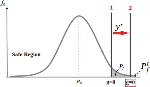
As in Figure 1, if the value of Pft is predefined, by shifting the limit state (g=0) from its original place to the location of line 2, the target failure probability will be obtained. This shift for limit state line can be done by means of an appropriate auxiliary shifting variable "y”.
The minimum value of y. is zero and begins from where the constraint g is zero (g=0). On the other hand, y can take a maximum value equal to the maximum value of g or the endpoint of the tail of PDF termed UBg
Figure 1.
Shifting the limit state line as much as an optimal valuey∗ to satisfy the desired reliability (Pft) for constraint g in probability space.
To calculate the required shifting for constraints, a very simple line search problem should be defined as
Minimize−ys.t.Pf−Pft≤00<y<UBgE4
Where the shifting variable "y” can only take values between 0 and upper bound of constraint distribution "g”. The amount of "y” should be maximized while the probability of failure is less than target failure probability. It states that seeking for a "y” is aimed so that the percentage of samples (of g’s distribution) that violates the value of "y” becomes equal to the target failure probability.
As it is stated in [4], as the design moves toward 100% reliability, the computational effort for searching the MPP in a standard normal space becomes greater. However, in the proposed approach, part of this issue is solved in the reliability assessment level by retrieving the useful historical data from nearby designs, and part of it can be addressed by relying on an adaptive "y” search strategy.
2.2 Adaptive shifting value search
If the value of y is chosen to be a very small amount, then the constraint will be shifted at a very low pace. Subsequently, the rate of convergence will decrease, and hence, after a great number of iterations the probability requirements would be met. On the other hand, if y takes a large value, it is very likely to have a premature design with higher reliability than is desired, meaning that an overdesign has occurred. To tackle this problem, an adaptive step size is introduced so as to make a tradeoff between the amount of constraint shifting and the level of required Pf . The essence is to move the design solution as quickly as possible to its optimum in order to eliminate the need for locating MPP that is adjusted to simulation-based approaches. The tradeoff problem is formulated as below:
Cost function=yratio+∆PfE5
yratio=yUBgE6
∆Pf=1N∑i=1NIinfdxi>yE7
Where the indicator function Iinf is defined as
IinfdX=1,x∈inf,0,else.
And xi,i=1,…,N are the N samples from probability distribution of constraint g. The first term in Eq. (5) denotes the normalized shifting value, and the second term denotes the error in failure probability.
The above problem can be stated in the form of a penalty function:
Cost function=yratio+r∑max0v2E8
and
v=1N∑i=1NIinfdxi>y−PftE9
Where multiplier "r” determines the severity of the punishment and must be specified a priori depending on the type of the problem (e.g., small failure problems).
The main advantage of using this penalty function is that in the initial iterations (less reliable designs), the shifting toward safe region would be quicker by putting more weight on "y”, whereas by approaching to the last iterations where the infeasible region becomes narrower, the second term of Eq. (5) outweighs the first term. Consequently, it does not allow for taking big step sizes and exceeding the Pft at later stages especially for rare events.
It should be noted that in Eq. (8), "r” plays the role of a controller to control the effect of the error term which should be changed adaptively. For instance, it can be stipulated that when the difference between Pf and Pftis less than an adequately small amount (e.g., 0.1), then an increase in the value of "r” will be applied, that is, magnifying the error in the failure probability. This is especially beneficial for the problems with stricter reliability requirements.
We use the results of the example 3.1 (section3) in advance for intuition.
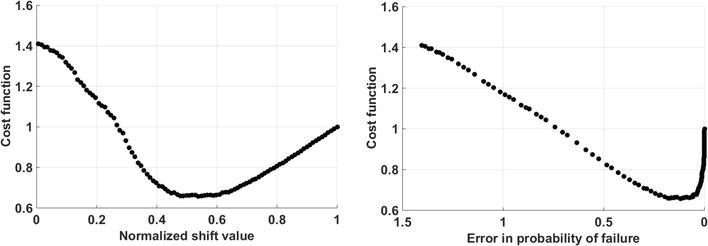
The value of "r” in the following problem is set to 1e+3 since the Pft is 1e−3. Accordingly, if the Pft was 1e-4, "r” should be set to 1e+4. To enlighten how the formula works, the tradeoff curve between the amount of shifting and the probability failure error is provided in Figure 2.
Figure 2.
Results of the adaptive optimal shift value search for example 1. The left panel indicates the effect of shift value step size on the cost function, and right panel indicates a sharp impact of error in the probability of failure on the cost function.
As is evident in Figure 2, by employing such optimization formulation, a tradeoff between two terms of the objective function is made; first, greater values of “normalized y” is in favor of minimizing the penalty function, because the great amount of failure probability has more impact on the penalty function and tries to make it maximum as fast as possible. Then, the trend will be reversed, meaning that the amount of shift becomes more important. Narrower failure region in the next iterations does not cause the effect of "y” to fade since "y” is normalized. The second term is squared so as not to allow any violation from Pft (occurrence of overdesign).
This shifting value search algorithm is robust because it is suitable for both continuous and discrete constraint functions.
Defining y and solving its optimization problem will not impose a significant computational load, because in fact, a comparison between a predefined value (Pft) and available samples is performed. As such, in each iteration a value for y is suggested which will be added to the deterministic constraint of the next iteration. Then, the DDO problem aiming at finding new optimal solution will be done considering the shifted constraint in a decoupled DDO-reliability assessment approach.
The algorithm will be in progress until a stopping criterion is satisfied. A proper stopping criterion for this framework could be a maximum shifting value or shifting vector (in case of more than one constraint). This criterion implies that constraints are all reliably satisfied. Therefore, by this search strategy adapted to simulation-based RBDO, the reliability of constraints improves progressively, while the need for searching MPPs is eliminated.
2.3 Sampling strategy for reliability analysis
To get an insight into the constraint’s behavior near the failure region, the first level of sampling (L1) is required. This will happen around the optimal point identified in the DDO of current iteration with the distribution properties defined for the random variables. Contrary to the existing sampling-based methods [30, 44], in the proposed method, for a more efficient sampling with least wastes, central limit theory is used. According to this theory, “the mean of a batch of samples will be closer to the mean of the overall population as the sample size increases” [45]. The overall population here means the huge MCS samples required to describe the probability distribution of the active constraints. Therefore, an adaptive sampling can be employed to distribute the initial samples around the optimal point of the current iteration regarding the difference between mean of the batch of samples and the mean of the whole population. By the aid of such adaptive sampling in each iteration, a more appropriate generation of sample size with less waste can be obtained. Moreover, this sampling will provide a distribution function for the constraint that has a better description of the failure region and hence provides a proper basis for the second-level sampling. The second-level sampling (L2) aims at distributing more samples with a focus on the region significant to the RBDO.
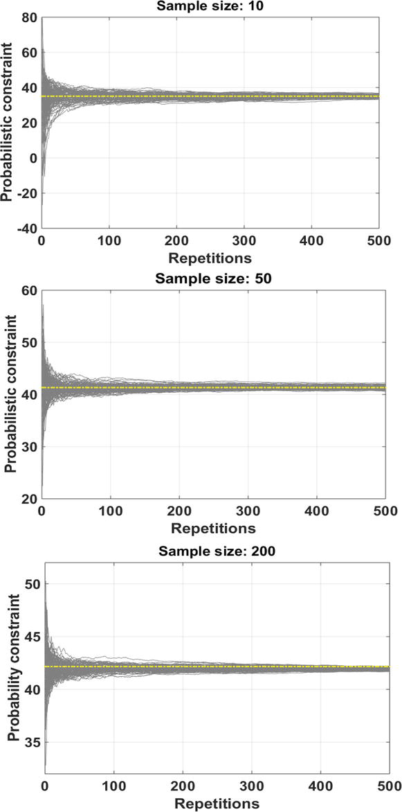
MCS has been run 500 times for example 1 (Section 3) to examine the process of convergence to the population mean (Figure 3). Then, it is repeated 100 times to exhibit the variability. In each run, a specified number of samples is generated, and then, these samples are aggregated with the previously produced samples. Then, the mean of the batches of samples is plotted in order to trace the value to which their means are approaching. Three different sample sizes are depicted to show the amount of variability for each one of them.
Figure 3.
Variability for different sample sizes in 500 repetitions of MCS.
Across the 500 repetitions, there was noticeable variability at low sample sizes. As expected, this variability decreases with larger sample sizes. Thus, in each RBDO iteration, an average sample size can be considered. Then, as long as the coefficient of variation (CoV) is not reached its desirable value, the process of generating the batch of samples will continue. In example 1 (Section 3), the sample size has been set to 50. The total number of samples generated to obtain a CoV of 0.1 was 1000 for the first iteration. It is clear that as the iterations continue, due to narrower failure region, more data is required. This volume of samples will be then adaptively determined based on the preset CoV. The impact of using CoV as the stopping criteria rule depends on the properties of the probability space. This adaptive initial sampling also reduces the potential error of improper sample size selection when building biasing density functions in IS methods.
Now, the generated samples will be used both for estimating the failure probability and the second level of sampling. In order to more accurately identify the constraint’s quantile of each cycle, two actions are taken; (1) Generating second level of sampling with its focus on the failure region, and (2) Recycling the historical samples (samples from previous iterations). For quantile-based failure probability, only the samples generated in the tail of the constraints are significant to an RBDO problem.
It goes without saying that initial sampling around the optimal point results in a number of samples dropped in the safe region and the rest dropped in the failure region. The latter are those carrying useful information for second level sampling.
It should be noted that once initial sampling is carried out, inactive constraints can be identified to avoid their contribution in second sampling. The strategy proposed by [46] can be employed to remove inactive constraints regardless of having knowledge about their boundaries.
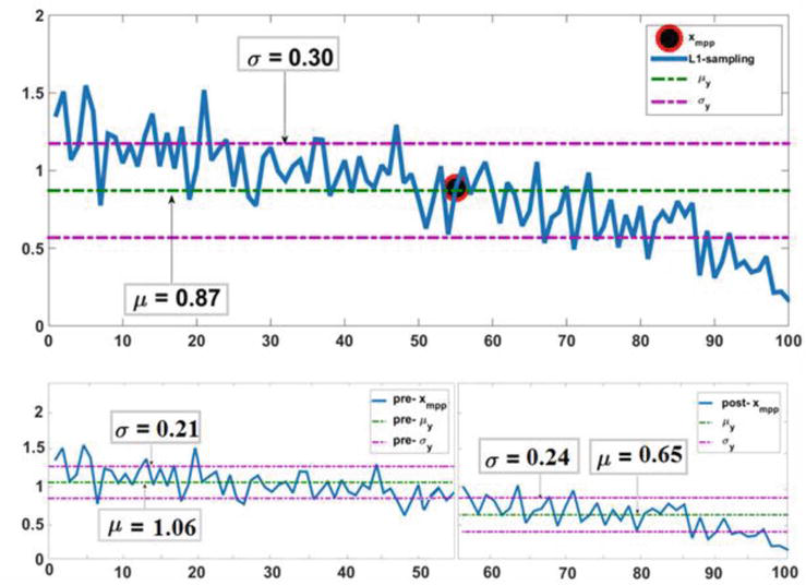
Figure 4 (top) shows the 100 random data generated from a normal distribution with mean of 0.87 and standard deviation of 0.3 in the L1. The location of xmpp is indicated as well. The panel has broken and classified the random samples to two parts: pre-xmpp and post-xmpp as are demonstrated in Figure 4 (bottom). So, there are two subsets of the main population of L1-sampling. It should be noted that regardless of the distribution types of random variables (i.e., normal, gumbel, weibull, etc.), to produce new samples, it is possible to safely use normal distributions. This is allowed by the central limit theorem [45].
Figure 4.
Top panel: Sample points generated for level one with a sample size of 100. Bottom panels: The same samples of upper panel but broken from the xmpppoint into two separate panels each with its own mean and standard deviation.
The standard deviation of the sampling distribution is smaller than the standard deviation of the population by a factor of √n [45], and hence, with this distribution, most of the L2-samples are distributed around the infeasible region.
Sorting the generated samples of random variables based on the index g=0 of constraint distribution gives the location of xmpp in the probability space.
Magnification of the infeasible region is subject to sufficient sampling from this region. Thus, new random samples will be generated with the mean and standard deviation of L1-samples dropped into the infeasible region (Figure 4, bottom right panel).
In failure probability estimation with IS, the smaller the variance of constructed biasing density, the more accurate the failure estimation. Chaudhuri et al. [30] have utilized the information reuse when building a posteriori biasing density to reach an optimal biasing density. Then, they sum the currently built biasing density with biasing densities of nearby designs to form the final density that will be used for failure probability estimation. In our proposed method, such strategy is employed but in a quantile-based frame to produce an accurate estimation of the failure probability. The newly generated samples along with the samples of the nearby design that have an overlap with the tail of current constraint’s distribution will form the final distribution function. Our method is different from [30] in the way the failure probability is calculated. In quantile-based method, the final distribution of the constraints will be directly used in the stage of searching for an optimal shifting value that is intended to reduce the failure probability error. In the implementation of the information reuse, no evaluation of the expensive LSF is required.
The new distribution function will be as below
gf=g+ginf+∑j=0k−1g´jE10
Where g is the initial distribution (from L-1 sampling), ginf is the distribution of L2-sampling, and g´j is the distribution built over all contributing samples from past RBDO iterations j∈0…k−1 that are stored in a database.
Similar to IS method where each sample has its own weight, in quantile-based method, each sample added to the g distribution causes a change in the MCS estimator. That is because by adding any single sample, the denominator in Eq. (7) will increase [42]. Thus, using the mixture distribution in the process of optimal shifting value search plays an important role in the accuracy of estimations.
Considering the recycled samples, L1-sampling and L2-sampling, the problem can be reformulated as
∆Pf=1nL1+nL2+m∑i=1nL1+nL2+mIinfdxi>yE11
Where the indicator function Iinf is defined as:
IinfdX=1,x∈inf,0,else.
Here inf.,, stands for the infeasible region of gfnL1nL2,m are the samples from gginf and g´j, respectively.
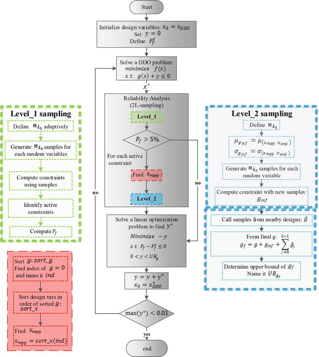
Figure 5 shows the flowchart of the proposed algorithm.
Figure 5.
Flowchart of the proposed algorithm.
In the next section, three well-known benchmark problems are employed to verify the efficiency and/or accuracy of the proposed method and to examine the whole proposed RBDO framework for quantile-based sampling methods.
In this section, the performance of the proposed framework in terms of applicability and computational efficiency will be investigated through three examples which are among widely cited benchmark problems. Then, the results will be compared with those previously presented for the sake of verification. To solve the deterministic optimization part, the sequential quadratic programming (SQP) through fminbnd function in MATLAB is used.
Since the computational cost of the deterministic optimization is negligible for sequential RBDO methods, the number of LSF evaluation (short form: NFE) is a fair measurement for efficiency.
The RBDO optimal solutions will be validated by using a crude MCS of ten million-size as a reference to satisfy the target failure probability.
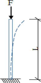
3.1 First RBDO problem: buckling of a straight column
A structural engineering problem is considered to practice both the efficiency and accuracy of the method. A long straight column with a rectangular cross section, fixed at one end and free at the other is considered (Figure 6) [47]. A deterministic axial load F is applied at the free end.
Figure 6.
A straight column with an axial load applied on it.
The column design optimization is defined so that the total area of the cross section should be minimized while the exerted load should not exceed the critical buckling load. This is formulated as below:
Minimizefx=bh
s.t.Pfx≤Pft
b−h≥0
gxp=π2Ebh312L2−Fa<0E12
Where b,h and p denote the width, the height of the column and random parameters, respectively. h,b are chosen to be the design variables.E, L and F stand for elasticity modulus, length of the column and axial load. Distribution information of E and L as random parameters and lower/upper bounds of b and h as deterministic variables are given in Table 1:
Variables
Distribution
Interval
Mean
CoV
bmm
Deterministic
[100,400]
—
—
hmm
Deterministic
[100,400]
—
—
FakN
Deterministic
1460
—
—
EMPa
Lognormal
—
10,000
0.15
Lmm
Lognormal
—
3000
0.15
Table 1.
Information on variables.
To examine the ability of the proposed algorithm to reach different target failure probabilities, three cases are considered (Table 2).
Results summarized for three cases with different Pft.
The results of Table 2 indicate that our algorithm not only is capable to satisfy the desired level of reliability but also compared to the other decoupled sampling-based method, uses less function calls. The algorithm has presented an efficiency of around 9, 5 and 2 times better in the first, second and third cases, respectively, in comparison with the other sampling method.
The probability of failure for the probabilistic constraint of each case at the optimum is evaluated by crude MCS with a ten-million sample points so as to ensure the target failure probability is not violated.
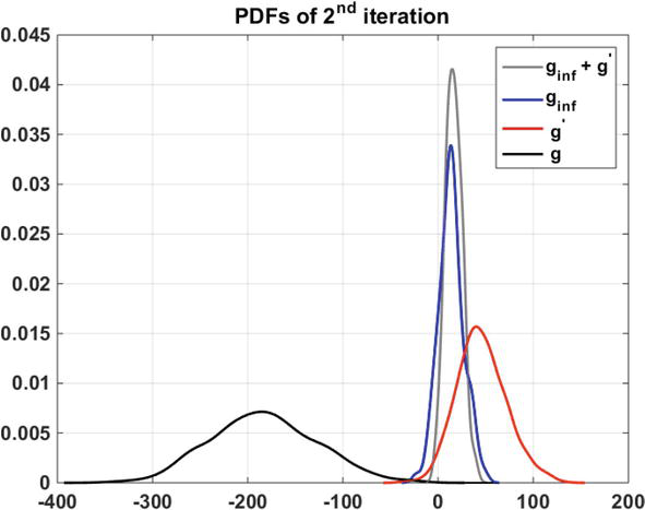
Calling samples of nearby design and generating samples with a focus on failure region has led to significant improvement in the effective samples of constraint’s quantile. The contribution of historical samples, L-1 sampling and L-2 sampling in the final distribution is 0.1%, 0.2% and 0.5% of the whole existing samples, respectively. Figure 7 is provided to illustrate the contribution of each batch of samples in the failure region.
Figure 7.
Pdfs of the kernel distribution fit to the random samples for second iteration(Pft=0.01) (example 1).
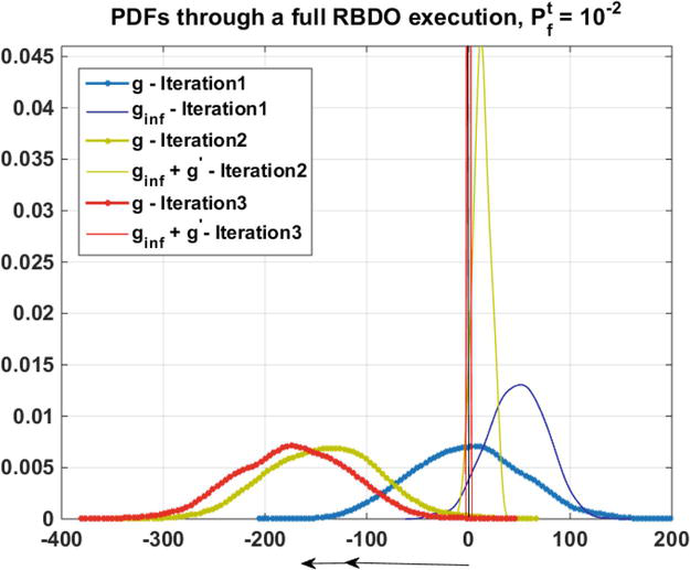
The amount of required shift for the constraint’s distribution within successive iterations to reach Pft=0.01 can be traced in Figure 8. It is obvious from Figure 8 that how the algorithm is able to shift the probability constraint to the safer region with respect to the required level of reliability. In each cycle, since the failure region at the tail of the probability constraint gets narrower, the contribution of the generated samples increases, while the contribution of the historical data from nearby designs drops.
Figure 8.
Pdfs of the kernel distribution fit to the random samples of all RBDO iterations for example 1 and for its second case (Pft=0.01).
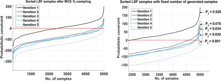
In case of setting a fixed sample size for all iterations and without recycling past information for the reliability analysis, the algorithm should produce much more samples to be able to converge to the reliable optimal point, and this will put an emphasis on the efficiency of the proposed sampling algorithm. As can be observed from Figure 9, without the defined adjustments in sampling levels, a sample size of 5000 is required in each iteration (a total of 25,000 for a full RBDO) to get the desired failure probability (Pft=0.001). However, with the measurements which are consistent with a quantile-based sequential RBDO, the total number of function evaluations is as few as 11,350, that is to say, 2.2 times less computational load without sacrificing the accuracy.
Figure 9.
A great number of samples, without the proposed strategy, required for each iteration to achieve the target failure probability (here Pft=0.001). Right panel is a zoomed view of the left panel (example 1).
3.2 Second RBDO problem: a highly nonlinear RBDO problem:
This problem is very well studied in various papers [48, 49], and the results of the proposed method are compared with an MCS-RBDO.
The considered mathematical design problem is formulated as
Minimizefx=−μx1+μx2−10230−μx1+μx2+102120
s.t.Pfgix>0≤Pf,it,i=1,2,3
g1x=1−x12x25
g2x=1−x1+x2−5230−x1−x2−122120
g3x=1−80x12+8x2+5E13
Which is a minimization problem including three nonlinear constraints. The input design variables x1and x2 are random with normal PDFs and standard deviation of 0.3 for each of them. The target failure probability is set to 2.28% for each constraint which is equivalent to 97.72%reliability. The deterministic optimal answer is taken as the initial point. The results are presented in Table 3.
The number in parenthesis of last column denotes results of the second run.
Youn et al. in [49] have pointed out that this problem could be a good benchmark example to be tested for RBDO methods because it has a highly nonlinear and nonmonotonic performance function g2 as one of the active constraints. Our proposed method has shown to have good stability in guiding the constraint boundaries toward their final locations. It is apparently observed that the proposed framework requires fewer LSF calls to reach the desired level of reliability. Therefore, it can save more computational efforts than a directional MCS-based RBDO algorithm.
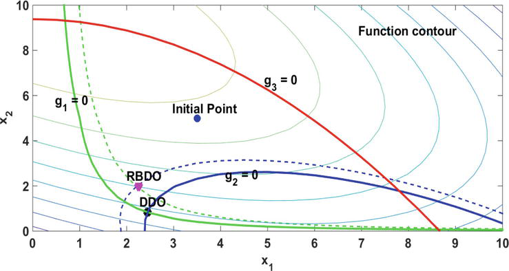
To give an insight into the deterministic and probabilistic constraints, Figure 10 illustrates the contours of the design space. The initial design point and the optimal points for DDO and RBDO are shown in this figure as well. The results of the first run (reported in Table 3) are obtained after three iterations. The iterations progress can be seen in Figure 11.
Figure 10.
Results of the proposed method in the design space, the boundaries of deterministic (solid lines) and probabilistic (dotted lines) constraints (example 2).
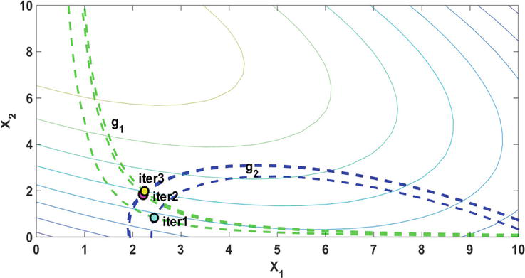
Figure 11.
Active constraints in three iterations and optimal points of each iteration (example 2). The final optimal point emerges in iteration 3.
The third constraint is not depicted in Figure 11 because the algorithm has removed the third constraint that was probabilistically inactive. The remaining active constraints are shifted in each iteration until the desired level of reliability is reached. The total amounts of shifting value for these active constraints are 1.171 and 0.166, respectively.
3.3 Third RBDO problem: highly nonlinear limit state with random and deterministic variables
This specific benchmark problem has been selected to investigate the convergence ability of the framework [50]. This problem is characterized by two normally distributed variables as well as two deterministic design variables in a highly nonlinear design space. This problem is mathematically expressed as Eq. (14). The first random variablex1has mean 5 and standard deviation 1.5, whereas the second variable x2 has mean and standard deviation equal to 3 and 0.9, respectively.
Findd=d1d2
Minimizefd=d12+d22
s.t.Prgxd≤0)≤φ−βt
0≤d1d2≤15
gxd=d1d2x2−lnx1E14
The optimization results of the proposed algorithm are reported in Table 4 alongside the reported result by Shayanfar et al. in [51] . With our proposed algorithm, the achieved optimal solution is [1.35, 1.35] which is consistent with the results obtained from methods RIA, PMA, SLA and SORA reported in [50] as well as with the particle swarm optimization-wolf search algorithm (PSO-WSA) proposed by Shayanfar et al. [51] (Table 4) are the same and all approaches converged to the optimal point [1.35, 1.35]. Our method is robust as it shows no sensitivity to the choice of the initial point. For example, the result of Table 4 is related to the initial point x0=45.
Optimization results of the proposed algorithm on the third RBDO problem in comparison with PSO-WSA.
Solving the DDO is dependent on the initial point, and this issue can cause problems when getting into the reliability assessment part. To reduce the dependency on the initial point, there was a need to choose an appropriate deterministic constraint handling. In order to make a balance between the effect of shift value and the error in failure probability, a cost function in the form of an exterior penalty function Eq. (8) is defined. This adjustment makes it possible for the algorithm to change the importance of the two terms adaptively, and hence, the dependency of the RBDO problem on the initial point is solved in this way.
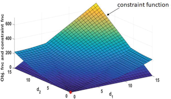
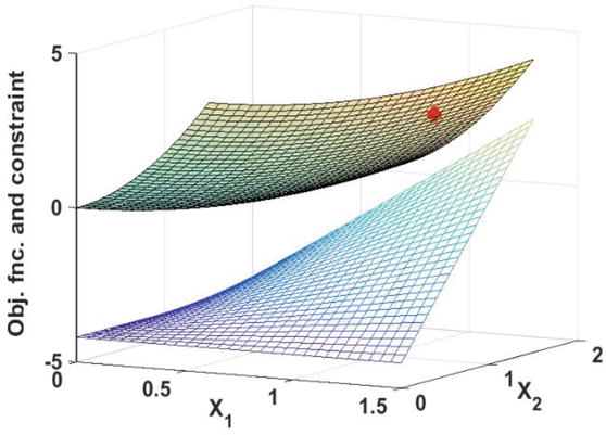
Figure 12 depicts a scheme of the objective function and constraint function in the allowed ranges of deterministic design variables.
Figure 12.
Design space of the third RBDO problem with the deterministic optimal point in red.
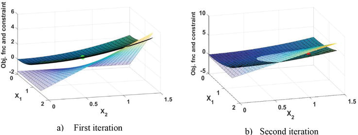
If the constraint is properly handled in the DDO problem, then from the first iteration the probabilistic constraint will be violated. Apart from sensitivity of solving the DDO, the reliability assessment also encounters difficulties from the moving direction of the constraint. When the algorithm is running, in each iteration a specified shifting value is added to the deterministic constraint. The optimal point in each iteration moves toward the safe region, due to the structure of the problem, shifting occurs in an inappropriate direction. Consequently, instead of increasing the solution's reliability, the algorithm faces an increase the failure probability. Figure 13 demonstrates the direction of moving constraint and optimal point for the first and second iterations. From this figure, it is clear that the optimal point has dropped into the infeasible region (Figure 13b.second iteration) due to the wrong direction.
Figure 13.
Design space of the third RBDO problem for two consecutive iterations.
This problem arises from the nonlinearity and the fact that there is no touch between the constraint function and the objective function at the points near the optimal solution. Some simple changes in the algorithm solve this issue such as replacing g+y with g−y in the optimization problem (Figure 5). Thereby, instead of reducing the failure probability, shifting values should be searched for which it leads to maximize the probability of success. In this case, necessary changes to the algorithm would be as the following:
Pf<5%→Psuccess>95%
Statistical properties of new samples for building ginf:
Mean: μsortxxmpp:xend→μsortxx1:xmpp
Std: σsortxxmpp:xend→σsortxx1:xmpp
gf>y→gf<−y
Pf=1N∑i=1NIinfdX
IinfdX=1,x∈inf≤−y,0,else.
Pft=5%→Psuccesst=95%
By making the above changes in the algorithm, the direction of shifting constraints will be reversed. See Figure 14.
Figure 14.
Design space of the third RBDO problem after making changes to reverse the direction of shifting constraint (last iteration).
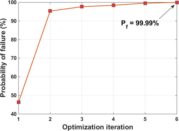
In Figure 15, as expected, the algorithm has sharply reached a high probability of failure at the very beginning when the reliability is still very low. Therefore, according to Eq. (5), the shift value term has outweighed the failure probability error. As the algorithm approaches the last iterations and hence the narrower the failure region, the algorithm performs the constraint’s shifting with smaller sizes until it minimizes the failure probability error. Another interesting point is that as opposed to many other sampling-based RBDO [30, 44], the proposed algorithm ensures a more reliable point in each iteration compared to previous iterations. According to Figure 15, the algorithm has converged from high errors in failure probability to lower errors as the algorithm progresses.
Figure 15.
Failure probability in each optimization iteration for the third RBDO problem.
Finally, from a top-down view, the proposed method has several advantages: First, due to adopting a sequential RBDO structure, only constraints which become active in each iteration will undergo reliability analysis which is not the case of double-loop methods. This causes a significant computational savings. Second, thanks to adopting sampling and quantile strategy in the estimation of failure probability, there is no need to struggle with searching a global MPP, particularly in highly nonlinear problems, as opposed to the existing sequential RBDO. Third, due to the adaptive step size introduced in the shifting value search strategy, we can make sure that a more reliable optimal point will be obtained in each iteration without any concern about the overdesign issue.
Table 5 is a general comparison between the proposed method and the existing methods which clearly show the applicability of the algorithm.
(In doing so, it is beneficial for high dimensional problems as well as nonlinear LSF especially for small failure probabilities and also non-Gaussian random variables.)
Construct surrogate models to estimate required objective functions?
Inspired by SORA’s method, a novel sequential RBDO method is proposed which integrates the shifting constraint’s strategy with quantile-based probability of failure estimation instead of MPP. Searching for global MPP is problematic when being performed in the random design space. Hence, in the proposed method, the RBDO structure is disintegrated in the probability space instead. This quantile-based algorithm uses a combination of different techniques to ensure a better result is obtained in each iteration so that wherever the problem is paused, it ensures us that the current design is more reliable than the previously generated ones. Once the deterministic optimization problem is solved, the failure probability estimation process in the probability space begins which is based on the quantile calculation with sampling. To enhance the computational efficiency in sampling, in the first level, the samples are generated adaptively. Then, the second-level sampling is done focusing on the failure region with the knowledge obtained from first-level sampling. Furthermore, the samples of previous iterations are reused to build a mixture distribution for which most of the samples are distributed in the failure region to provide an accurate estimate of the quantile. After the quantile is calculated, with an efficient adaptive step size for the optimal shifting value, the algorithm is able to quickly converge to the target failure probability. We explored the efficiency of the proposed method through three benchmark problems. The results show that the proposed method will decrease the computational cost to less than half of what is reported about other existing methods in very small target probabilities (Pft=0.001) and down to 9% in mild target probabilities (Pft=0.1 and Pft=0.01)). It is also able to provide promising results both for highly nonlinear problems and problems with mixture of normal–nonnormal variables as well as random-deterministic variables. As an extension to this work, the same framework will be combined with the IS concept to reach a potentially more efficient algorithm for smaller failure probabilities, and we will explore it in the future works.
This work was conducted with the support of the Science Foundation Ireland Centre for Research Training in Artificial Intelligence under Grant No. 18/CRT/6223.
No potential conflict of interest was reported by the author(s).
References
1.Beck AT, Gomes WJS, Bazán FAV. On the robustness of structural risk optimization with respect to epistemic uncertainties. International Journal for Uncertainty Quantification. 2012;2(1):1-20
2.Lopez RH, Beck AT. Reliability-based design optimization strategies based on FORM: a review. Journal of the Brazilian Society of Mechanical Sciences and Engineering. 2012;34:506-514
3.Tu J, Choi KK, Park YH. A new study on reliability-based design optimization. Journal of Mechanical Design. Dec 1999;121(4):557-564 (8 pages)
4.Du X, Chen W. Sequential optimization and reliability assessment method for efficient probabilistic design. Journal of Mechanical Design. 2004;126(2):225-233
5.Agarwal H et al. An inverse-measure-based unilevel architecture for reliability-based design optimization. Structural and Multidisciplinary Optimization. 2007;33(3):217-227
6.Torii AJ, Lopez RH, Miguel LFF. On the accuracy of reliability index based approaches and its application to RBDO problems. In: 22nd International Congress of Mechanical Engineering (COBEM 2013), Brazil. 2013
7.Kuschel N, Rackwitz R. Two basic problems in reliability-based structural optimization. Mathematical Methods of Operations Research. 1997;46(3):309-333
8.Huang ZL et al. An incremental shifting vector approach for reliability-based design optimization. Structural and Multidisciplinary Optimization. 2016;53(3):523-543
9.He Q et al. Reliability and multidisciplinary design optimization for turbine blade based on single-loop method. Tuijin Jishu/Journal of Propulsion Technology. 2011;32(5)
10.Liang J, Mourelatos ZP, Tu J. A single-loop method for reliability-based design optimization. In: International design engineering technical conferences and computers and information in engineering conference. 2004; 46946
11.Jiang C et al. An adaptive hybrid single-loop method for reliability-based design optimization using iterative control strategy. Structural and Multidisciplinary Optimization. 2017;56:1271-1286
12.Meng Z et al. Convergence control of single loop approach for reliability-based design optimization. Structural and Multidisciplinary Optimization. 2018;57:1079-1091
13.Keshtegar B, Hao P. Enhanced single-loop method for efficient reliability-based design optimization with complex constraints. Structural and Multidisciplinary Optimization. 2018;57(4):1731-1747
14.Yao W et al. Review of uncertainty-based multidisciplinary design optimization methods for aerospace vehicles. Progress in Aerospace Sciences. 2011;47(6):450-479
15.Madsen H, Krenk S, Lind N. Methods of Structural Safety. Englewood Cliffs: Prentice-Hall; 1986
16.Melchers RE, Beck AT. Structural Reliability Analysis and Prediction. UK: John Wiley & Sons; 2018
17.Lee SH, Kwak BM. Response surface augmented moment method for efficient reliability analysis. Structural Safety. 2006;28:261-272
18.Rahman S, Xu H. A univariate dimension-reduction method for multi-dimensional integration in stochastic mechanics. Probabilitic Engineering Mechanics. 2004;19:393-408
19.Youn BD, Zhimin X. Reliability-based robust design optimization using the eigenvector dimension reduction (EDR) method. Structural and Multidisciplinary Optimization. 2009;37:475-492
20.Au SK, Beck JL. A new adaptive importance sampling scheme for reliability calculations. Structural Safety. 1999;21(2):135-158
21.Kanj R, Joshi R, Nassif S. Mixture importance sampling and its application to the analysis of SRAM designs in the presence of rare failure events. In: Proc. Design Autom. Conf., ACM, 2006
22.Au S-K, Beck JL. Estimation of small failure probabilities in high dimensions by subset simulation. Probabilistic Engineering Mechanics. 2001;16(4):263-277
23.Elsheikh A, Oladyshkin S, Nowak W, Christie M. Estimating the probability of CO2 leakage using rare event simulation. In: ECMOR XIV-14th European conference on the mathematics of oil recovery. 2014
24.Shayanfar MA et al. An adaptive directional importance sampling method for structural reliability analysis. Structural Safety. 2018;70:14-20
25.Li H-S, Cao Z-J. Matlab codes of Subset Simulation for reliability analysis and structural optimization. Structural and Multidisciplinary Optimization. 2016;54(2):391-410
26.Li HS, Ma YZ. Discrete optimum design for truss structures by subset simulation algorithm. Journal of Aerospace Engineering. 2015;28(4):04014091
27.Yu T, Lu L, Li J. A weight-bounded importance sampling method for variance reduction. International Journal for Uncertainty Quantification. 2019;9(3)
28.Li L, Bect J, Vazquez E. Bayesian subset simulation: A kriging-based subset simulation algorithm for the estimation of small probabilities of failure. In: 11th International Probabilistic Assessment and Management Conference (PSAM11) and The Annual European Safety and Reliability Conference (ESREL 2012), Helsinki: Finland. 2012. arXiv:1207.1963
29.Au SK, Wang Y. Engineering Risk Assessment with Subset Simulation. Singapore: John Wiley & Sons; 2014
30.Chaudhuri A, Kramer B, Willcox KE. Information reuse for importance sampling in reliability-based design optimization. Reliability Engineering & System Safety. 2020;201:106853
31.Motamed M. A multi-fidelity neural network surrogate sampling method for uncertainty quantification. International Journal for Uncertainty Quantification. 2020;10(4):315-332
32.Zhao Y, Lu W, Xiao C. A kriging surrogate model coupled in simulation-optimization approach for identifying release history of groundwater sources. Journal of Contaminant Hydrology. 2016;185-186:51-60
33.Mi X, Zhang J, Gao L. A system active learning Kriging method for system reliability-based design optimization with a multiple response model. Reliability Engineering & System Safety. 2020;199:106935
34.Jiang C et al. Global and local Kriging limit state approximation for time-dependent reliability-based design optimization through wrong-classification probability. Reliability Engineering & System Safety. 2021;208:107431
35.Ciriello V, Di Federico V, Riva M, Cadini F, De Sanctis J, Zio E, et al. Polynomial chaos expansion for global sensitivity analysis applied to a model of radionuclide migration in a randomly heterogeneous aquifer. Stochastic Environmental Research and Risk Assessment. 2013;27(4):945-954
36.Gao T, Li J. A cross-entropy method accelerated derivative-free RBDO algorithm. International Journal for Uncertainty Quantification. 2016;6(6):487-500
37.Zhao W, Qiu Z. An efficient response surface method and its application to structural reliability and reliability-based optimization. Finite Elements in Analysis and Design. 2013;67:34-42
38.Yang I-T, Hsieh YH. Reliability-based design optimization with cooperation between support vector machine and particle swarm optimization. Engineering with Computers. 2013;29(2):151-163
40.Alyanak E, Grandhi R, Bae H-R. Gradient projection for reliability-based design optimization using evidence theory. Engineering Optimization. 2008;40(10):923-935
41.Wang Z, Song J. Cross-entropy-based adaptive importance sampling using von Mises-Fisher mixture for high dimensional reliability analysis. Structural Safety. 2016;59:42-52
42.Li G, Yang H, Zhao G. A new efficient decoupled reliability-based design optimization method with quantiles. Structural and Multidisciplinary Optimization. 2020;61(2):635-647
43.Yi P, Xie D, Zhu Z. Reliability-based design optimization using step length adjustment algorithm and sequential optimization and reliability assessment method. International Journal of Computational Methods. 2019;16(07):1850109
44.Beaurepaire P et al. Reliability-based optimization using bridge importance sampling. Probabilistic Engineering Mechanics. 2013;34:48-57
45.Fischer H. A History of the Central Limit Theorem: from Classical to Modern Probability Theory. Springer Science & Business Media; 2010
46.Chen Z, Li X, Chen G, Gao L, Qiu H, Wang S. A probabilistic feasible region approach for reliability-based design optimization. Structural and Multidisciplinary Optimization. 2017
47.Liu W-S, Cheung SH. Reliability based design optimization with approximate failure probability function in partitioned design space. Reliability Engineering & System Safety. 2017;167:602-611
48.Kim D-W et al. A single-loop strategy for efficient reliability-based electromagnetic design optimization. IEEE Transactions on Magnetics. 2015;51(3)
49.Youn BD, Choi KK, Du L. Enriched performance measure approach for reliability-based design optimization. AIAA Journal. 2005;43(4):874-884
50.Aoues Y, Chateauneuf A. Benchmark study of numerical methods for reliability-based design optimization. Structural and Multidisciplinary Optimization. 2010;41(2):277-294
51.Shayanfar MA, Barkhordari MA, Roudak MA. An efficient reliability algorithm for locating design point using the combination of importance sampling concepts and response surface method. Communications in Nonlinear Science and Numerical Simulation. 2017;47:223-237
Written By
Shima Rahmani, Elyas Fadakar and Masoud Ebrahimi
Reviewed: February 9th, 2023Published: March 9th, 2023